21.1 Finite Difference Algorithms#
Definitions#
By definition, Finite Differencing is a method to approximate partial differential equations which we cannot solve, into a system of algebraic equations which we can.
Notation to simplify our representations:
- Superscripts: We use superscripts to denote steps in the time domain \( t^n = n \Delta t \). Here \( n = [0, N] \) is the step index and \( \Delta t \) is the time-step \( T/N \)
- Subscripts: \( x_j = j \Delta x \). Here \( j = [0, J] \) is the step index and \( \Delta x = L/J \) is the spatial step.
- Together: \( u_j ^n = u(t^n, x_j) \)
- Explicit algorithms: Use data that is already known at the present time to advance the solution to the next time step. They are easier and faster to implement, but they introduce stability constraints.
- Implicit algorithms: Use data from the next time step when advancing the solution. Leads to a system of equations that must be solved simultaneously
One look at the typical definition of the derivative suggests an algebraic approximation
\[\dv{f}{x} = \lim_{\Delta x \rightarrow 0} \frac{f(x + \Delta x) - f(x)}{\Delta x} \quad \rightarrow \quad \dv{f}{x} \approx \frac{f(x + \Delta x) - f(x) }{\Delta x}\]Applying to our model equation, the linear advection equation
\[\pdv{u}{t} + c \pdv{u}{x} = 0\]The first-order forward difference approximation for the temporal derivative is
\[\pdv{u}{t} \approx \frac{u_j ^{n+1} - u_j ^n}{\Delta t} \equiv \Delta _t u\]And the first-order backward approximation for \( \pdv{u}{x} \) is
\[\pdv{u}{x} \approx \frac{u_{j} ^n - u_{j-1} ^n}{\Delta x} \equiv \nabla _x u\]These are sometimes called Euler differencing, since they are first-order. Plugging in our approximations, we arrive at the “Forward Euler Algorithm”
\[\frac{u_{j} ^{n+1} - u_j ^n}{\Delta t} + c \frac{u_{j} ^n - u_{j-1} ^n}{\Delta x} = 0\]This is an explicit scheme: solve for \( u^{n+1} _j \)
\[u_j ^{n+1} = u_j ^n - \frac{c \Delta t}{\Delta x} (u_j ^n - u_{j-1} ^n)\]The multiplier out front \( \frac{c \Delta t}{\Delta x} \) is very important for stability, so we call it
\[\frac{c \Delta t}{\Delta x} = \text{ Courant number (or CFL number)}\]For the problem to be mathematically well-posed, we must know initial conditions and boundary conditions
\[u(t = 0, j) \qquad u(t, x = 0)\]Accuracy#
We can be more precise with the error in our difference approximation: the error will be on the order of \( \Delta x \):
\[\dv{f}{x} \approx \frac{f(x + \Delta x) - f(x) }{\Delta x}\] \[\rightarrow \dv{f}{x} = \frac{f(x + \Delta x) - f(x) }{\Delta x} + O(\Delta x)\]As it turns out, we can improve the accuracy of the finite difference operators by using centered differences:
\[\left. \pdv{u}{x} \right|_{j} = \frac{u_{j+1} ^n - u_{j-1} ^n}{2 \Delta x} + O(\Delta x ^2)\]So the forward-time, centered-space (FTCS) PDE becomes
\[\frac{u_j ^{n+1} - u_j ^n}{\Delta t} + c \frac{u_{j+1} ^n - u_{j-1} ^n }{2 \Delta x} = 0\]This is more accurate than the Euler method in space. We can write the accuracy as \( O(\Delta t, \Delta x^2) \), or “it is first-order accurate in time and second-order accurate in space.”
How do we get accuracy estimates? The accuracy is defined by using a Taylor series expansion for the finite-difference operators:
\[u_j ^{n+1} = u_j ^n + \pdv{u}{t} \Delta t + \frac{1}{2} \pdv{ ^2 u}{t^2} \Delta t^2 + \frac{1}{6} \pdv{ ^3 u}{t ^3} \Delta t^3 + \ldots\] \[u_{j+1} ^n = u_j ^n + \pdv{u}{x} \Delta x + \frac{1}{2} \pdv{ ^2 u}{x^2} \Delta x^2 + \frac{1}{6} \pdv{ ^3 u }{x ^3} \Delta x ^3 + \ldots\] \[u_{j-1} ^n = u_j ^n - \pdv{u}{x} \Delta x + \frac{1}{2} \pdv{ ^2 u }{x^2} \Delta x^2 - \frac{1}{6} \pdv{^3 u }{x^3} \Delta x ^3 + \ldots \]Substituting into the Forward Euler algorithm:
\[u_j ^n + \pdv{u}{t} \Delta t + \frac{1}{2} \pdv{^2 u }{t^2} \Delta t^2 + \frac{1}{6} \pdv{ ^3 u}{t ^3} \Delta t^3 + \ldots\] \[= u_j ^n - \frac{c \Delta t}{\Delta x} \left( u_j ^n - \left[ u_j ^n - \pdv{u}{x} \Delta x + \pdv{^2 u }{x^2} \frac{\Delta x ^2}{2} \pm \ldots \right] \right)\]After simplifying and re-arranging/canceling like terms, we get
\[\pdv{u}{t} + c \pdv{u}{x} = - \frac{1}{2} \pdv{^2 u}{t^2} \Delta t - \frac{1}{6} \Delta t^2 + \ldots + \frac{c}{2} \pdv{^2 u}{x^2} \Delta x - \frac{c}{6} \pdv{ ^3 u }{x ^3} \Delta x ^2 + \ldots\]The left-hand side is the PDE we’re trying to solve, so everything on the right-hand side is the error term introduced by our approximation. The solution we’re going to get is actually the solution to the modified PDE with all of the error terms. Reading off the lowest-order terms of \( \Delta x \) and \( \Delta t \) we see that the algorithm is first-order accurate in space and time.
Algorithm Requirements#
For an algorithm to work, it requires the following properties:
- Consistency: Whatever finite difference operator \( \delta_x u \) we use, applied to our solution, has to approximate the derivative as the spacing goes to zero
- Stability: The solution must be bounded, so for some initial condition \( u \) the norm goes to zero as the number of points goes to infinity
- Accuracy: The accuracy is bounded by the finite difference operator
- Convergence: The numerical solution must approach the exact solution as the grid spacing goes to zero
A useful theorem is Lax’s Theorem: An algorithm that is consistent and stable will converge. This means that we only have to prove consistency, stability, and accuracy.
Consistency#
Let’s take our Forward Euler algorithm as an example: From analyzing the accuracy, we derived the modified PDE and noted the leading-order error terms. Forward Euler gave \( O(\Delta x, \Delta t) \). As \( \Delta t, \Delta x \rightarrow 0 \), we recover the original PDE. Therefore, FE is consistent.
Likewise the FTCS is also consistent, since \( \Delta t, \Delta x \rightarrow 0 \) also recovers the original PDE. In fact, because the accuracy of FTCS was \( O(\Delta x ^2, \Delta t) \) it is also consistent.
Stability#
The way to perform the stability analysis is to use Fourier transforms to convert from a discrete spatial domain to a continuous frequency domain. Broadly speaking, the mathematical tools we have at our disposal to analyze stability only apply to continuous functions - you can’t take a derivative of a set of discrete points. By transforming to a continuous domain, we can use properties of our basis functions to examine the growth of errors over time. This process is called Von Neumann Stability Analysis.
Example: Stability analysis of FTCS
\[u_j ^{n+1} = u_j ^n - \frac{a \Delta t}{2 \Delta x} \left( u_{j+1} ^n - u_{j-1} ^n \right)\]We define an error norm by subtracting the exact solution
\[\varepsilon_j ^n = u_j ^n - \overline{u}\] \[\varepsilon_j ^{n+1} = \varepsilon_j ^n - \frac{a \Delta t}{2 \Delta x} \left( \varepsilon_{j+1} ^n - \varepsilon_{j-1} ^n \right)\]To study the evolution of the errors, apply a Fourier transform to get to frequency space:
\[\varepsilon_j ^n = V^n e^{ik_x x} = V^n e^{ik_x (j \Delta x)}\] \[V^n = \text{ wave amplitude}\] \[k = \text{ wavenumber } = \frac{2 \pi}{\lambda_x}\]Substituting,
\[V^{n+1} e^{i k_x j \Delta x} = V^n e^{i k_x j \Delta x} - \frac{a \Delta t}{2 \Delta x} \left(V^n e^{i k_x (j+1) \Delta x } - V^n e^{i k_x (j-1) \Delta x} \right)\] \[\rightarrow \frac{V^{n+1}}{V_n} = 1 - \frac{a \Delta t}{2 \Delta x} \left( e^{i k_x \Delta x} - e^{-ik_x \Delta x} \right)\]The ratio \( V^{n+1}/V^n \) tells us how the amplitudes of the errors will evolve in time. We define the amplification factor \( G \)
\[G = \left| \frac{V^{n+1}}{V^n} \right|\]For stability, we need the errors not to grow over time, so the Von Neumann stability criterion is:
\[G^m \leq 1 \quad \forall n\]Continuing with our example
\[\frac{V^{n+1}}{V_n} = 1 - \frac{a \Delta t}{2 \Delta x} \left[ \cos (k_x \Delta x) + i \sin(k \Delta x) - \cos (-k_x \Delta x) - i \sin (- k_x \Delta x) \right]\] \[= 1 - i \frac{ a \Delta t}{\Delta x} \sin (k_x \Delta x)\]To get the amplification factor, we need the norm
\[G = \left[ \left(1 - i \frac{ a \Delta t}{\Delta x} \sin (k_x \Delta x) \right) \left( 1 + i \frac{ a \Delta t}{\Delta x} \sin (k_x \Delta x)\right) \right] ^{1/2}\] \[= \sqrt{ 1 + \left(\frac{a \Delta t}{\Delta x}\right)^2 \sin ^2 (k_x \Delta x)}\]But that’s always greater than 1! So FTCS is unconditionally unstable.
Performing the same analysis for Forward Euler, we get a stability condition:
\[0 \leq 1 + 2\frac{a \Delta t}{\Delta x} \left( \frac{a \Delta t}{ \Delta x} -1 \right) (1 - \cos (k_x \Delta x)) \leq 1\]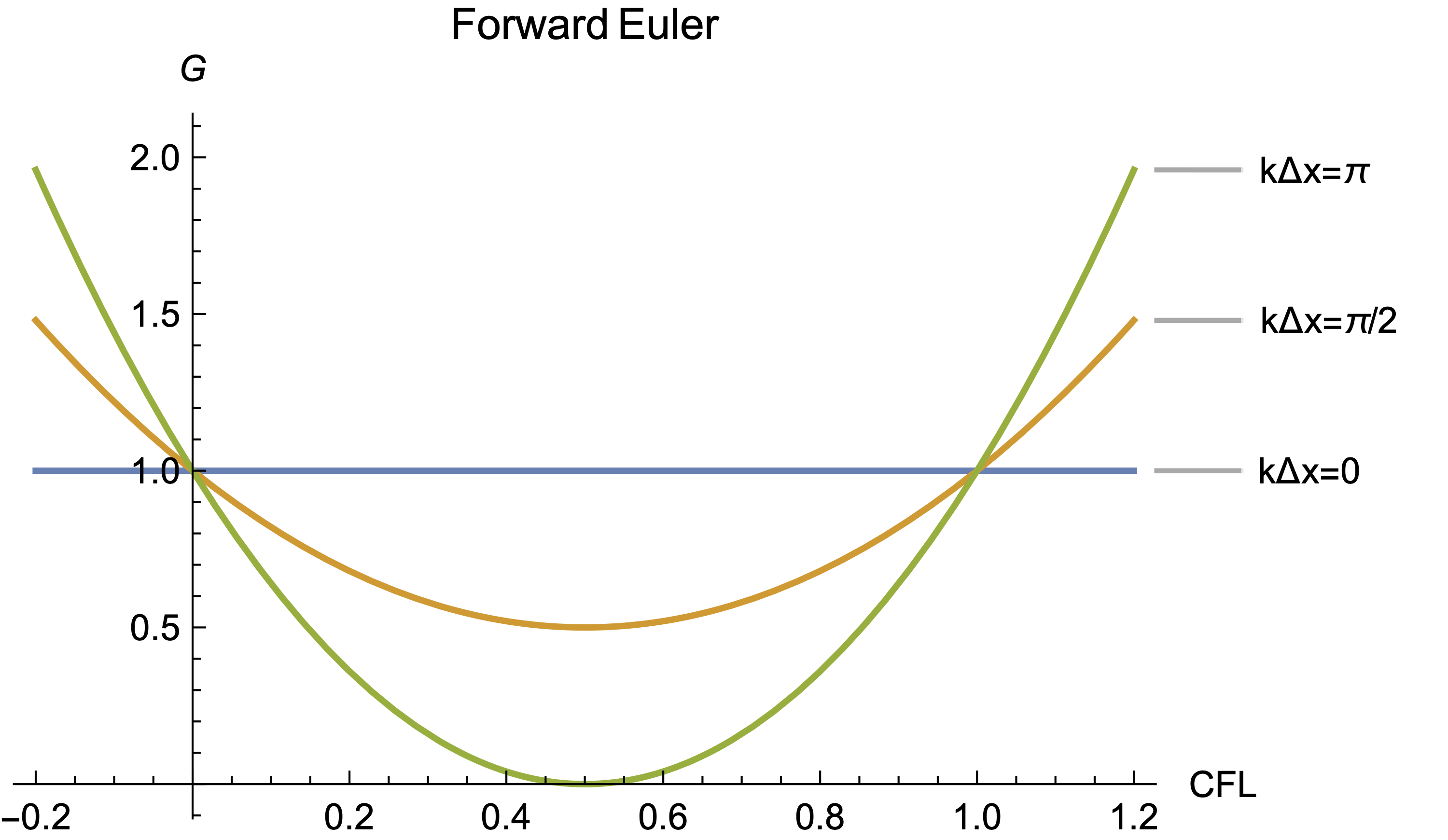
We can see that the CFL number must be
\[0 \leq \frac{a \Delta t}{\Delta x} \leq 1\]Possible values of \( k_x \Delta x = \frac{2 \pi}{\lambda} \Delta x \) . The minimum of \( k_x \Delta x \) occurs at \( \lambda = \infty \), uniform error throughout the domain. This only occurs if the error is everywhere zero, since the boundary conditions are presumed accurate. In practice, the maximum wavelength is equal to twice the length of the domain
\[\lambda_{max} = 2L\] \[(k_x \Delta x)_{max} = \frac{\pi}{J-1}\]The maximum of \( k_x \Delta x \) is for \( \lambda = 0 \), but this is not possible on a grid with finite grid points. The Nyquist limit tells us that \( \lambda_{min} = 2 \Delta x \). That means that
\[(k_x \Delta x)_{max} = \pi\]When you violate a stability condition, what do we expect to see? The error growth is largest for the largest value of \( k_x \Delta x \), which corresponds to a wavelength equal to the grid spacing. In practice, that looks like errors that blow up from point to point.
Convergence#
We want to show that the numerical solution approaches the exact solution to the original PDE.
Lax’s equivalence theorem states:
If an algorithm is consistent and stability requirements are satisfied, the numerical solution will converge to the solution of the original PDE.
This is why consistency and stability is so important; if you have both, then you have convergence, which tells you that the problem you’re solving is the problem you are actually trying to solve.
Accuracy#
The solution exists at discrete locations for multiple variables, e.g \( \rho, p, u, v, \ldots \), so we want a convenient measure of solution accuracy.
The general p-norm is defined as
\[\text{p-norm} = L_p = \left[\sum_{j=1} ^J |z|^p \right]^{1/p}\]In practice, the most common norms that we use are the 1, 2, or \( \infty \)-norms.
\[L_1 = \sum |z| \quad \text{(average)}\] \[L_2 = \left[ \sum |z|^2 \right]^{1/2} \quad \text{(variance)}\] \[L_{\infty} = \text{max}|z| \quad \text{(max-norm)}\]In practice, the 2-norm is the most rigorous definition of the error. Specifically, we define the error norm in the form
\[\text{Error norm} = \left[ \sum_{j=1} ^{J} \Delta x ( \varepsilon) ^2 \right] ^{1/2} = \sqrt{\Delta x} || \varepsilon ||_2\] \[\varepsilon_j = u_j - \overline{u}\]Sources of Errors?#
Where do errors come from? In order to reduce our model’s error, we must first understand where the errors come from.
Truncation errors - Result from the terms in the Taylor series difference approximation that are neglected. They can be reduced by using higher accuracy difference operators.
Round-off errors - Result of the limited machine accuracy (accuracy of floating point representation). It can be reduced by using higher precision to store values, or by performing fewer calculations.
Bugs - Don’t have bugs. ha. ha. ha. But really, we can minimize programming errors through practices like good planning, good comments, etc.