Plasma Models #

First, let’s get a working definition of “plasma”: “a quasi-neutral gas of charged and neutral particles that exhibit collective behavior.” Many of the approaches we will describe will also apply to non-neutral plasmas. Plasmas are composed of particles (electrons, ions, neutrals) which interact through electric and magnetic fields and through collisions. Therefore, the plasma can be modeled as individual particles.

Plasmas exhibit collective behavior due to the long-range forces from EM field interactions. As a consequence of this collective behavior, the plasma can alternately be modeled as an electrically conducting fluid. These seemingly conflicting models can be married together by taking a statistical approach to convert from particles to a continuous distribution, or by defining fluid elements to treat as particles.

We will see that these statements are partially correct and partially incorrect. The accuracy of a particular sort of model depends on the length scales and time scales of interest, which are themselves determined by the plasma parameters. Consider a typical tokamak plasma which has a lifetime on the order of \( 10^2 \) seconds and electron plasma period on the order of \( 10^{-12} \) seconds. The physical dimensions are on the order of \( 1 m \) with a Debye length of \( 10^{-5} m \). We have quite a large range of parameters to handle!

Sometimes the large range of scales allows a separation between “fast” and “slow” dynamics, but generally this presents a challenge because the scales interact with each other (challenging multi-scale problem). At very fast time scales, the slower effects can be roughly approximated as equilibria.

Hierarchy of Plasma Time Scales #

In broad terms, we can define a hierarchy of plasma time scales.

• \( \omega_{pe} \) \( (10^{-12} s) \) If we consider the fastest time scale, we think of the electron plasma frequency. It is associated with high frequency electromagnetic waves (~light speed). Associated with this time scale, but perhaps a little slower, we have electron dynamics, wave propagation (both electrostatic and electromagnetic).

• \( \omega_{p, i} \) \( (10^{-9} s) \) The next-fastest time scale is the ion plasma frequency. It is associated with ion oscillations, which become important in magnetized plasmas where electrons can move along magnetic fields in response to charge separation.

• \(k v_A (10^{-9} - 10^{-6} s) \) Ion cyclotron waves: electrostatics (Bernstein waves), electromagnetic (Alfvén waves)

• \(k v_s (10^{-6}s) \) Ion acoustic waves

• \( \omega ^\star (10^{-4}s) \) Drift waves (\( \omega ^\star = \) drift frequency \( \approx \grad p_e / e B n \))

• \( (k v_a \nu)^{1/2} (10^{-3}s) \) Collisional effects (resistivity): magnetic reconnection, tearing instabilities, plasma disruptions

• \( (\sim s) \) Energy and plasma confinement time scales, including transport phenomena, which depend on effects from shorter time scales, and drift waves

Hierarchy of Plasma Models #

We can define a hierarchy of plasma models, which does not correspond directly with the hierarchy of time scales, but is related.

N-Body Model #

In an N-body model, each particle is treated classically. Particles interact through the Lorentz force and collisions. We usually limit collisions to binary collisions, but we don’t have to. Electromagnetic fields are generated by particle positions and particle motion. The equation of motion looks like this:

The collision term only involves collisions between two particles. As we said, we’re limiting collisions to binary collisions. The delta function comes from the assumption of infinitesimally small point particles.

To solve the model, we just track each particle \( (\vec r_i, \vec v_i) \) in a Lagrangian frame of reference. In a Lagrangian frame of reference, we track each individual particle in its own frame of reference, as opposed to a lab frame or cell frame.

The particles couple to the fields as source terms to the Maxwell equations.

Maxwell’s equations give \( \vec E \) and \( \vec B \) at each particle’s position \( r_i \)

More generally we can write a Hamiltonian description

where \( p \) is the generalized momentum and \( v \) is the generalized position. If the system is conservative, we can define \( \mathcal{H} \) such that:

From this, we can write a statement of conservation of phase space, called the Klimontovich equation:

where the particle phase space is given by

The total number of particles in a typical lab plasma is \( \sim 10^{21} \). Each particle interacts with every other particle, which gives a number of interactions \( \sim 10^{42} \). Implementation of the full N-body model is impractical. If we perform an ensemble average of the very spiky Klimontovich equation, we arrive at a statistical description (the Liouville equation) for the probability distribution function, \( f(\vec x, \vec v, t) \). This results in an expression that looks like this:

Now we’re summing over coordinates, not particles. The RHS “cross terms” describe the collisional terms, which leads to the BBGKY hierarchy.

We can also express the Liouville equation in a general way as the Boltzmann equation:

This describes the evolution of the probability distribution function \( f \). We must compute the Boltzmann equation for each species \( \alpha \):

For small plasma parameters \( (n \lambda_D ^3)^{-1} \) and no collisional effects, the collisional terms vanish and we have the Vlasov equation:

The advantage of using a continuous distribution \( f \) instead of the discrete particle description is that we can directly compute the various derivatives. This is a continuum description, like a fluid but in phase space.

Phase Space Kinetic Model - Continuum Kinetic Model #

We can evolve \( f_\alpha (\vec x, \vec v) \) directly in 6D space by coupling Maxwell’s equations with the Vlasov equation

\( \rho \) and \( j \) are the sources for the Maxwell equations. With the evolution of \( \vec E \) and \( \vec B \) in hand, we are free to compute all terms in the Vlasov equation (Vlasov-Maxwell Model).

For numerical implementations, it is usually advantageous to write the equation to be solved in “conservation form”

If collisions are important, then solve Boltzmann-Maxwell model. The conservation law form of the Boltzmann equation is

This is called a “weakly conservative” form, because the right-hand side is not equal to zero. We can also write out Maxwell’s equations in conservative form, and combine them with Boltzmann to get the full conservation form of the Boltzmann-Maxwell model.

If we assume collisions are small angle scatterings and large angle scattering results as multiple small angle scatterings, then the collision terms can be truncated.

\[\left. \pdv{f}{t} \right|_{coll} = \pdv{}{\vec v} \left( \left\langle \frac{\Delta \vec v}{\Delta t} \right\rangle f \right) + \frac{1}{2} \pdv{}{\vec v} \pdv{}{\vec v} \dot \cdot \left( \left\langle \frac{ \Delta \vec v \Delta \vec v}{\Delta t} \right\rangle f \right) \] \[= \sum_i \pdv{}{v_i} \left( \frac{\Delta v_i}{\Delta t} f \right) + \frac{1}{2} \sum_{j, k} \pdv{}{v_j} \pdv{}{v_k} \left( \langle \frac{\Delta v_j \Delta v_k}{\Delta t} \rangle f \right)\]

where \( F(\vec v \rightarrow \vec v + \Delta \vec v) \) is the probability that a particle’s velocity changes from \( \vec v \) to \( \vec v + \Delta \vec v \) in a time \( \Delta t \). Since any particle must have a velocity after \( \Delta t \), the \( F \) is normalized such that

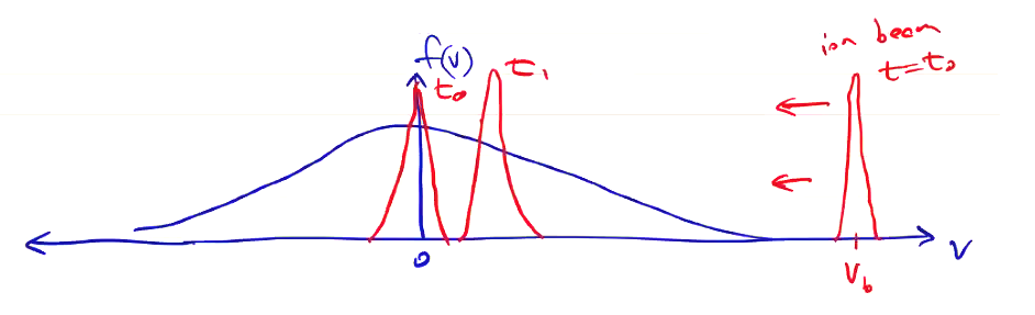
The first term of the Fokker-Planck collision operator \( \pdv{}{\vec v} \left( \left\langle \frac{\Delta \vec v}{\Delta t} \right\rangle f \right) \) represents the slowing down of particles due to collisions with slower moving particles. For example, consider a beam injected into a stationary plasma. Assuming the beam is dense (i.e. it is not affected by the plasma), the distribution function is composed of a stationary distribution centered about \( v=0 \), and a narrow distribution centered at the beam velocity. Over time, the collision operator will act to drive the centroids together. Intuitively, it has a frictional effect:

Moving on to the second term,

this represents the heating of particles due to collisions with a hotter population. It will tend to drive the variances (temperature) together, and so acts as a velocity diffusion term:

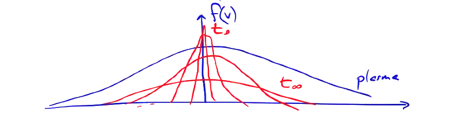
The Fokker-Planck collision model is one of the most complicated forms that can actually be computationally solved, and gives a pretty good description of most laboratory and astrophysics plasmas.

The Boltzmann H-theorem tells us that “\( f \) will tend towards a Maxwellian as a result of collisions.” This suggests that simpler forms of the collision operator can be found which maintain the characteristics of the full Fokker-Planck operator, but are easier to solve. One such operator is the BGK operator:

where \( f_M \) is a Maxwellian distribution with the same first three velocity moments (\( n, \vec u, T \)) as \( f \), and \( \tau \) is a relaxation time.

In this sense, the BGK collision operator is a relaxation operator (towards a Maxwellian) of the Fokker-Planck collision model.