Particle-In-Cell Model (Particle model revisited)#
The order of magnitude issues with the N-body model prevent a direct application in even simple laboratory plasmas. In a plasma with \( N = O(10^{21}) \), we have interactions on the order of \( O(10^{42}) \) making direct computation completely impractical.
We can instead use representative particles with the same charge to mass ratio, but fewer (\( N = 10^3 \sim 10^7 \)) particles. The governing equations for such a model look very similar to the N-body model:
\[\dv{\vec v_i}{t} = \left( \frac{q}{m} \right)_i (\vec E + \vec v_i \cross \vec B) + \sum_{j \neq i} \left. \dv{\vec v_{ij}}{t} \right|_{coll} \delta (\vec r_i - \vec r_j)\] \[\dv{\vec r_i}{t} = \vec v_i\]
These hold for each superparticle \( i \). We can track the position and velocity in time \( (\vec r, \vec v)_i \) of each superparticle \( i \). The physical properties of superparticle \( i \) will be:
\[m_i = m_\alpha \frac{N_{plasma}}{N_{model}} \qquad \alpha = \text{ion, electron, ...}\] \[q_i = q_\alpha \frac{N_{plasma}}{N_{model}}\] \[n_i = n_\alpha \frac{N_{model}}{N_{plasma}}\]Since \( q_i / m_i = q_\alpha / m_\alpha \), the collisionless dynamics will be preserved for the same \( \vec E \) and \( \vec B \). Provided a sufficiently large number of superparticles (adequate statistics), this means we can use this heavily reduced model to capture the entire behavior of the plasma.
Let’s compute some plasma parameters for this “undersampled” system.
\[\omega_p = \sqrt{\frac{n_\alpha q_\alpha ^2}{\epsilon_0 m_\alpha}} = \sqrt{\frac{n_i q_i ^2}{\epsilon_0 m_i}}\]We find that the plasma frequency remains the same for the sampled system. The cyclotron frequency is also preserved for the physical system.
\[\omega_c = \frac{q_\alpha B}{m_\alpha} = \frac{q_i B}{m_i}\]However, if we look at the Debye length, we see that it changes
\[\lambda_D = \frac{v_{th}}{\omega_p} = \sqrt{\frac{\epsilon_0 k T_\alpha}{n_\alpha q_\alpha ^2}} = {\sqrt{\frac{\epsilon_0 k T_i}{n_i q_i ^2}}} \sqrt{\frac{N_{model}}{N_{plasma}}}\]This difference will have important implications on the spatial scales and resolution of the model. The coupling to the Maxwell’s equations is accomplished as we did in the N-body model.
There are two outstanding issues that we need to address before we can move on to computation:
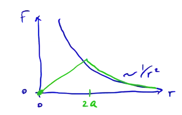
- Singularities. The Coulomb force between two charged particles approaches \( \infty \) as \( r \rightarrow 0 \).
- Large number of interactions. Even with fewer particles, \( O(10^7) \), there are still \( N^2 \) particle-particle interactions at all times. \( O(10^{14}) \) interactions is still not really practical to compute.
To deal with singularities, we can use finite-size particles, with their properties diffusely distributed throughout their volume. When these particle “clouds” begin to overlap, the overlapping volumes cancel each other, and when the particles overlap entirely (\( r = 0 \)), the force is zero
The same technique is used in hydrodynamics in a model called SPH (smooth particle hydrodynamics). SPH techniques are used quite often for hypervelocity impacts, like asteroids striking a planet. An interesting application of SPH is the brasil nut problem: why do brasil nuts end up at the top of a can of mixed nuts? As it turns out, if we model simple normal collisions in a can of particles of varying sizes, we don’t see the effect at all. However, if we introduce friction between particles then the effect does show up, so we can deduce that the surface area to volume ratio of the brasil nut is important.
Using SPH in a plasma is more complicated, because plasma particles interact with every other particle through long range EM forces. We can no longer limit interactions locally in a plasma. Instead, to limit the number of interactions, we use a spatial grid to integrate the EM forces. Electromagnetic sources from each particle \( i \) are assigned to a spatial grid node \( j \)
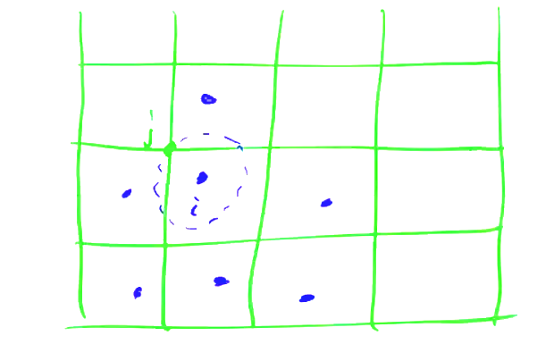
Then, \( \vec E \) and \( \vec B \) are computed on the grid based on \( \rho_j \) and \( \vec j _j \) to give \( (\vec E, \vec B)_j \). Then, particle positions and velocities are evolved using \( (\vec E, \vec B)_j \) to compute local forces on each particle.
The computational time required to compute the fields depends on the number of grid points, \( M \). At each time step, this requires \( O(M^2) \) operations. The computational time required to compute assign particles positions and velocities to the grid and compute forces on each particle is \( O(N) \). This makes the total compute time \( O(M^2 + \alpha N) \ll N^2 \)
Relationship to N-Body and Kinetic Models#
PIC is similar to the N-body model in some obvious ways:
- The plasma is treated as discrete particles that interact through EM fields
- Same governing equations, only with fewer particles
However, the EM fields are computed by currents and charges localized to a spatial grid. This is an important distinction. It is what removes the n-body interactions from the model.
By comparison to the kinetic model, kinetic models are derived by performing an ensemble average to transform from discrete space to a smooth, continuous space. The averaging process accounts for smoothly varying long-range forces, which is just what we’ve done by mapping our particles to a spatial grid. The short-range abrupt forces are encompassed in the collision operator in the same way. The same idea of separating the smooth long-range forces from the abrupt forces was the key Vlasov insight. As we arbitrarily crank up the spatial resolution, the PIC model converges not to the N-body model, but to the Vlasov kinetic model.
PIC models are “particle ensemble averages,” but not in a strict sense. They can be thought of as a sampling or discretization of the continuous phase space.
General Comments on Kinetic Models#
- The PIC method is a robust and efficient method for collisionless plasmas. Collisions are usually modeled using Monte Carlo methods.
- PIC does not work well when the physics is dominated by a small population (small number of particles), because the sampling error becomes very significant.
- PIC methods work well for handling vacuum boundaries, but physical boundaries are more difficult. This is the opposite of the case for fluid models.
- PIC methods naturally resolve sharp features in phase space, e.g. a cold beam
- Continuum kinetic methods can require more computational effort. PIC methods have been around since the 60’s, but continuum models have only become computationally practical more recently. There are a couple of reasons for this. Dimensionality is a key component. Continuum distribution methods encompass a six-dimensional space, but particle methods can work in three-dimensional spaces. Additionally, solving the governing equations Boltzmann, Vlasov, Vlasov + Fokker-Planck, etc. are more complicated than the equation of motion for the PIC method.
- Continuum methods better model tails of distributions, which is often where interesting physics happens. E.g ionization, fusion are driven by the high energy tail of the distribution, while the overall dynamics are determined by the bulk. If tails are not interesting, then computational effort is wasted on large unoccupied regions of phase space. Tails also constrain the numerical solution for continuum methods. High velocity and low density can lead to oscillations where the value of the distribution function is very small, leading to potentially negative values.
- Continuum methods (more generally fluid methods) can introduce numerical diffusion and dispersion.
- Diffusion leads to a smoothing of sharp features over time.
- Dispersion leads to low/high wavenumber features propagating at the wrong speed.
Computational Methods for PIC#
- PIC can easily be extended to include relativistic effects, only requiring minimal changes to the equation of motion.
- Collisions are often neglected in PIC methods, assuming a low density, collisionless plasma. As we try to apply PIC methods to collisional plasmas, the accuracy gets worse.
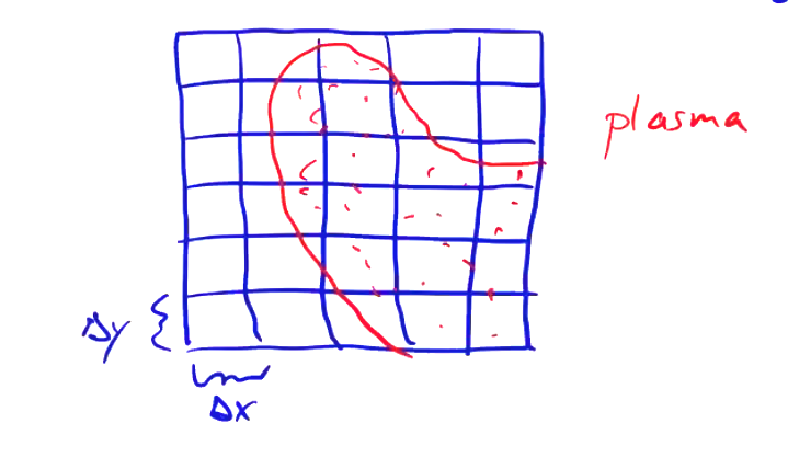
Let’s talk about how we go about solving the governing equations for a plasma. First, we divide the domain into a uniform grid, \( \Delta x = \Delta y = \Delta z = const. \). We will have a distribution of particles throughout the domain with independent position and velocity \( (\vec x, \vec v)_i \).
The geometry of the particles themselves depends on dimensionality.
- Particles have an infinite extent in unresolved dimensions. In 3D, this means that particles are spheres. In 2D they are cylindrical, and in 1D they are planar.
The general procedure for solving the PIC method goes like this:
- Particles are weighted to the grid. The position of each particle \( i \) in phase space \( (\vec x, \vec v)_i \) is weighted to the grid to compute the electromagnetic source terms \( (\rho_c, \vec j)_j \) at each grid location \( j \). \[\underbrace{(\vec x, \vec v)_i}_{\text{particles}} \rightarrow \underbrace{(\rho_c, \vec j)_j}_{\text{grid}} \qquad \text{(Particle weighting)}\]
- Advance the electric and magnetic fields on the grid \[\underbrace{(\rho_c, \vec j)_j}_{\text{grid}} \rightarrow \underbrace{(\vec E, \vec B)_j}_{\text{grid}} \qquad \text{(Field solve)}\]
- Electromagnetic fields are weighted to particles \[\underbrace{(\vec E, \vec B)_j}_{\text{grid}} \rightarrow \underbrace{\vec F_i}_{\text{particle}} \qquad \text{(Force weighting)}\]
- Particles are advanced in time \[\vec F_i \rightarrow \vec v_i \rightarrow \vec x_i\]
Particle & Force Weighting#
As mentioned earlier, PIC uses finite size particles rather than point particles to avoid the issue of force singularities. This is particularly important in the 1-dimensional case, since infinitesimal particles would never be able to exchange positions. The exact size and shape of the particles matter. The charge density for a point particle is
\[\rho_c(\vec r) = q_i \delta (\vec r - \vec r_i)\]For a finite-size particle,
\[\rho_c (\vec r) = q_i S(\vec r - \vec r_i)\]where \( S \) is a particle shape factor. Conservation of charge requires \[\int S(\vec r - \vec r_i) \dd \vec r = \int \delta ( \vec r - \vec r _i) \dd \vec r = 1\]
The Lorentz force must be weighted to the particles using the same shape factor in order to get consistent dynamics. For \( \vec B = 0 \), \[\vec F_i = q_i \vec E (\vec r_i) = \overbrace{q_i \int \vec E(\vec r) \delta (\vec r - \vec r_i) \dd \vec r}^{\text{point particles}} \\ = \underbrace{q_i \int \vec E(\vec r) S(\vec r - \vec r_i) \dd \vec r}_{\text{finite-size particles}}\]
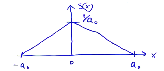
Particles must have local support, meaning \( S(\vec r - \vec r_i) \) is spatially restricted to a small portion of the grid. The simplest weighting/shape is a uniform charge cloud. In 1D, this is
\[S(x) = \begin{cases} 1/a_0 &\qquad & \text{if} \quad |x| \leq a_0 /2 \\ 0 &\qquad & \text{otherwise} \end{cases}\]This provides zeroth-order weighting to the nearest grid point (NGP). When we go to compute the fields from our source terms, the particle will only contribute to the closest single grid point.
If the size of our particle is very small compared to the grid spacing \( \Delta x > a_0 \), what happens to \( \rho_c \) as the particle drifts through the grid? Because we compute the weighted density as \( \rho_c (\vec r) = q_i S(\vec r - \vec r_i) \), there will be some positions for which a particle will not contribute to any grid point. Likewise, if \( \Delta x < a_0> \), then the particle appears on multiple grid points, but only at some times, producing double-counting. Both of these cases violate conservation of charge:
\[\pdv{}{t} \int q_\alpha f_\alpha \dd \vec x \dd \vec v = 0\]To conserve charge, \( \Delta x \) must equal \( a_0 \). This is a limitation of zeroth-order weighting.
Even if we have \( \Delta x = a_0 \), nearest grid point still produced particles that appear and disappear on the grid instantaneously, but at least they appear/disappear in a way that conserves total charge. The resulting charge distribution is noisy as a result, hinting at a general issue with PIC methods. The noise introduced by weighting charge distribution to a grid is addressed by using many particles, \( N \gg M \). Typically, we’ll use \( N \sim M^2 \).
The nearest grid point weighting can be improved to 1st order, using a linear \( S(x) \).
We maintain the important property \( \int S(x) \dd x = 1 \). Using \( a_0 = \Delta x \) so that
\[\sum_j S(x_j - x) = 1\]for any \( x \). The resulting charge density after weighting looks like this:
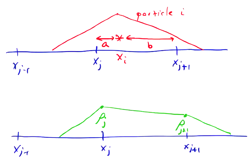
The same weighting strategy extends to multiple dimensions. In 2D, this is bilinear weighting; in 3D we have trilinear. 1st order weighting requires more computational effort than nearest grid point, but produces smoother fields. The instantaneous appearance/disappearance of particles as they move across the grid is now gone, leading to a smoother electric field. This is the typical PIC weighting method. Higher-order weightings further reduce noise, but with dramatically increased computational expense. For example, a second-order scheme might be
\[S_2( x_j - x) = \frac{3}{4} - \left( \frac{x - x_j}{\Delta x} \right)^2\] \[S_2(x_{j \pm 1} - x) = \frac{1}{2} \left( \frac{1}{2} \pm \frac{x - x_j}{\Delta x} \right) ^2\]
All shape functions must satisfy conservation of charge \( \sum_j S(x_j - x) = 1 \) for any \( x \). But they must also preserve the first moment
\[\sum_j x_j S(x_j - x) = x\]to preserve the electric dipole moment. And, of course, we require \( S(x) \geq 0 \) everywhere. This last requirement will trip up higher order methods if we naively use Lagrange interpolation functions. Instead, we can construct higher orders by using functions defined by convolutions of lower order shapes.
\[\begin{aligned} m = 1 & \qquad & S _{NGP} \star S_{NGP} = \int S_0(x') S_0 (x - x') \dd x' = S_1(x) \\ m = 2 & \qquad & S_1 \star S_{NGP} = S_x(x) \end{aligned}\]As you go to higher and higher order, \( S_m(x) \) approaches a Gaussian.
Let us consider, does the particle shape affect the field distribution? What about the force distribution? Consider a uniform, finite-size ion and an infinitesimal electron (sheet), such that \( q_i + q_e = 0 \).
\[\int e n_i \dd x + \rho _s = 0\]From Gauss’s law,
\[\dv{E_x}{x} = \frac{\rho_c}{\epsilon_0}\]with \( E_x = 0 \) outside. Solving Gauss’s law, we find an electric field like this:
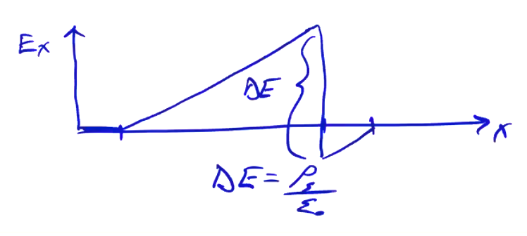
From this, we conclude that outside of the particle extent, the field is independent of the particle shape. If we consider a charge sheet with an arbitrary shape \( \rho_c(x) \) in an electric field, bounded between \( x = a, x = b \), the force on the sheet is
\[F = \int_a ^b \rho_c (x) E_x \dd x = \int_a ^b \frac{\epsilon_0}{2} \dv{}{x} (E_x ^2) \dd x \\ = \frac{\epsilon_0}{2} (E_b ^2 - E_a ^2) = \epsilon_0 (E_b - E_a) \left( \frac{E_b + E_a}{2} \right) = \epsilon_0 \Delta E \overline{E} = q \overline{E}\]The particle shape does not affect the physics outside of the particle shape. The force on the particle is only determined by the average electric field.
Particle Push#
Once the source terms have been weighted to the grid, we wish to advance particles’ position and velocity based on the Lorentz force.
\[m \dv{\vec v}{t} = \vec F \\ \dv{\vec x}{t} = \vec v\]We could solve these using any time integration technique, e.g. Runge-Kutta. But instead, we are going to choose a leap-frog method. It requires the fewest operations for the same order of accuracy (2nd order) and is a symplectic integrator, which means that it is a canonical transformation from one time to another time. Canonical transformations have important conservation properties; symplectic integrators conserve integrators, and are reversible in time.
To push the particles, we will use finite difference operators to approximate the ODEs.
\[m \frac{\vec v^{new} - \vec v^{old}}{\Delta t} = \langle \vec F \rangle \\ \frac{\vec x^{new} - \vec x^{old}}{\Delta t} = \langle \vec v \rangle\]The averaging treatment we use to get the RHS determines the numerical accuracy and stability of the scheme.
\[\vec v^{new} = \vec v^{old} + \frac{\Delta t \langle F \rangle}{m} \\ \vec x^{new} = \vec x^{old} + \Delta t \langle \vec v \rangle\]Here is where the leap-frog method comes in. We will center the right-hand side in time to get a 2nd order accuracy. By off-setting the velocity and position calculations, we get the average velocity we need for the centered leap-frog:
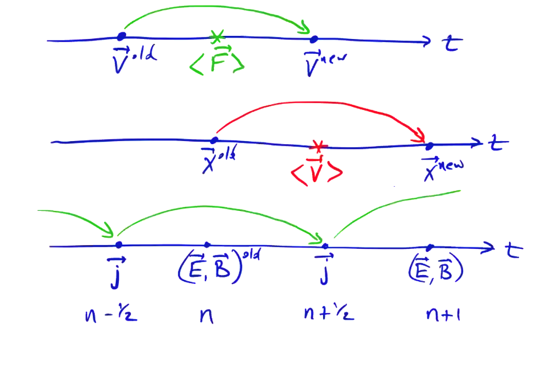
To properly center the force, \( \vec E \) and \( \vec B \) must be expressed at the same points as position. They are then used to compute the next velocity \( v(n+1/2) \), from which we advance the position.
Leap-frog is second order accurate, but can be dispersive. This will give us incorrect wave speeds/frequencies/phase, but correct magnitude. Consider an electrostatic harmonic oscillator (Langmuir oscillations). For a charged particle oscillating around a fixed particle,
\[\frac{v^{n + 1/2} - v^{n-1/2}}{\Delta t} = \frac{q}{m} E(x^n)\] \[\frac{x^{n+1} - x^n}{\Delta t} = v^{n+1/2} \qquad \text{ and } \qquad \frac{x^n - x^{n-1}}{\Delta t} = v^{n-1/2}\]
Gauss’s law gives
\[\dv{E}{x} = \frac{q n }{\epsilon_0} \rightarrow E(x^n) = \frac{q n }{\epsilon_0} x^n\]Combine to give
\[\frac{x^{n+1} - 2 x^n + x ^{n-1}}{\Delta t^2} = \frac{q}{m} E(x^n) = - \frac{q^2 n}{m \epsilon_0} x^n = - \omega_p ^2 x^n\]This equation approximates the ODE for Langmuir oscillations
\[\dv{^2 x}{t^2} + \omega_p ^2 x = 0\]which has the solution
\[x(t) = C e^{\pm i \omega_p t}\]That’s the same finite difference we’re using for our leap-frog particle push, which indicates that we’re solving the same differential equation. We can assume an oscillating solution to our finite difference equation where
\[x^n = c e^{i \omega t^n}\]where \( t^n = n \Delta t \). Substituting \( x^n \) into the finite difference expression, \[e^{i \omega \Delta t} - 2 + e^{- i \omega \Delta t} = - \omega _p ^2 \Delta t^2\]
Some algebraic manipulation leads to
\[2\left( \frac{e^{i \omega \Delta t} + e^{- i \omega \Delta t}}{2} - 1 \right) = - \omega_p ^2 \Delta t^2 \\ 2 \left( \cos (\omega \Delta t) - 1 \right) = - \omega _p ^2 \Delta t^2\\ \sin ^2 \left( \frac{\omega \Delta t}{2} \right) = \left( \frac{\omega _p \Delta t}{2} \right)^2\]That’s interesting. We should have a solution \( \omega = \pm \omega_p \), but instead we have this other solution. Plotting \( (\omega \Delta t / 2) \) vs \( (\omega_p \Delta t / 2) \), we get a plot like this:
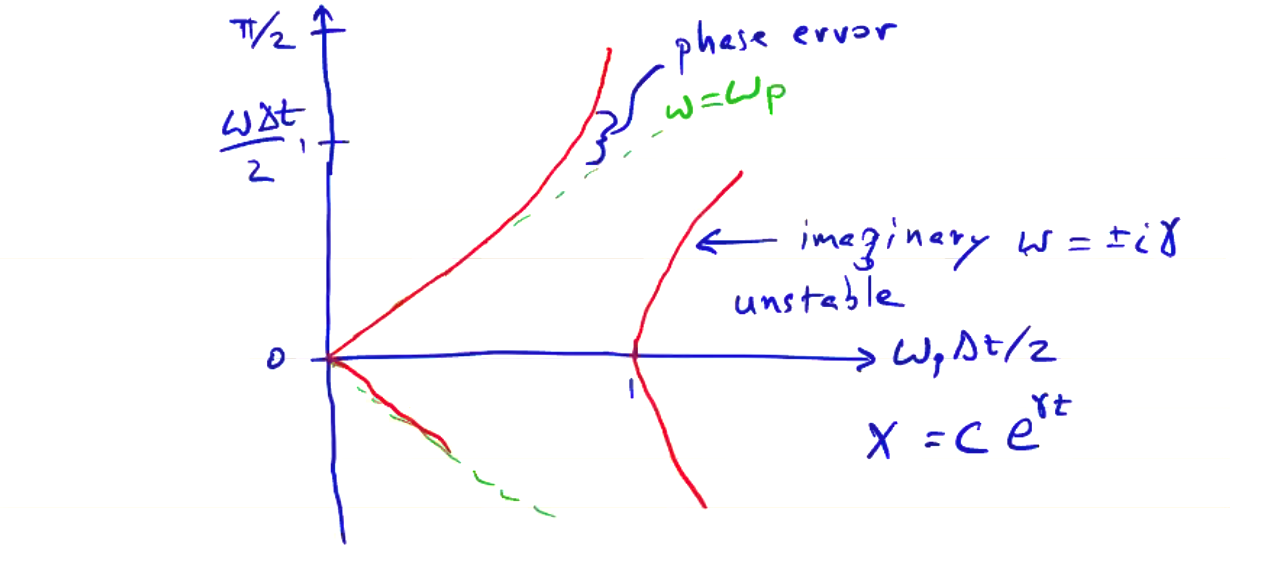
The deviation from \( \omega = \omega_p \) is what’s called a phase error. Nominally, we can set \( \Delta t \) to whatever we want. Setting \( \Delta t \) further out gives an imaginary \( \omega = \pm i \gamma \), so
\[x = c e^{\gamma t}\]which is an unstable solution. So, if \( \Delta t \) is small, the leap frog finite difference gives an accurate solution. Increasing \( \Delta t \) enters a region where phase errors become large. Going all the way up to \( \Delta t = 2/\omega_p \), we get imaginary solutions to the differential equation and the solution becomes unstable. This is the Leap-frog instability.
Electromagnetic Field Solver#
At the field solver step, we need to advance \( \vec E \) and \( \vec B \) according to Maxwell’s equations based on particles’ positions and velocities.
In the electrostatic case, Faraday’s law reduces to \[\curl \vec E = 0 \rightarrow \vec E = - \grad \phi\]
Combined with Gauss’s law, yields Poisson’s equation
\[\div \vec E = \rho_c / \epsilon_0 \rightarrow \grad ^2 \phi = - \rho_c / \epsilon_0\]Poisson’s equation can be solved with finite differences. In 1D,
\[\frac{\phi _{j+1} - 2 \phi_j + \phi_{j-1}}{\Delta x^2} = - \frac{\rho_j}{\epsilon_0}\]In matrix form, this yields a tridiagonal matrix equation.
\[\vec A \vec \phi = \vec b \rightarrow \vec \phi = \vec A ^{-1} \vec b\]where
\[\vec \phi = \begin{bmatrix} \phi_1 \\ \phi_2 \\ \vdots \\ \phi_J \end{bmatrix}\] \[\vec A = \frac{1}{\Delta x^2} \begin{bmatrix} \ldots & 1 & -2 & 1 & \ldots \end{bmatrix}\] \[\vec b = \begin{bmatrix} - \rho_{j-1} / \epsilon_0 \\ - \rho_j / \epsilon_0 \\ \rho_{j+1} / \epsilon_0 \\ \ldots \end{bmatrix}\]We can run into some trouble here with periodic domains. For a periodic boundary condition, \( \vec A \) looks like
\[\vec A \sim \begin{bmatrix} -2 & 1 & 0 & \\ 1 & -2 & 1 & \\ \ldots & \ldots & \ldots & \ldots \\ \ldots & 1 & -2 & 1 \\ 1 & \ldots & 1 & -2 \\ \end{bmatrix}\]which is singular. This problem arises from a lack of appropriate boundary conditions. Even with periodic boundary conditions, we know the solution \( \phi \) is lacking an appropriate gauge, e.g. \( \phi_1 = 0 \) or \( \sum_j \phi_j = 0 \). Setting \( \phi_1 = 0 \) modifies \( \vec A \):
\[\vec A \sim \begin{bmatrix} 1 & 0 & 0 & \\ 1 & -2 & 1 & \\ \ldots & \ldots & \ldots & \ldots \\ \ldots & 1 & -2 & 1 \\ 1 & \ldots & 1 & -2 \\ \end{bmatrix}\]This is no longer singular, and we can invert it.
With \( \phi_j \) in hand, we compute the electric field as
\[E_{x_{j}} = - \frac{\phi_{j+1} - \phi_{j-1}}{2 \Delta x}\]and solve the Vlasov-Poisson system.
Periodic Domains - Fourier Series Expansion#
For periodic domains, an alternative approach to solving Poisson’s equation has some unique advantages compared to the finite difference method. In this approach, we transform from a discrete physical space to Fourier wave space. In wave space, differential operators become multiplications.
\[\rho(x) \overbrace{\rightarrow}^{FT} \rho(k)\]using the transformation kernel \( e^{i k x} \). Poisson’s equation becomes
\[k ^2 \phi (k) = \rho(k) / \epsilon_0 \rightarrow \phi(k) = \frac{\rho(k)}{\epsilon_0 k^2}\]With the potential, an inverse fourier transform gives \( \phi(k) \rightarrow \phi(x) \). We can get the field either by computing the gradient
\[- \grad \phi(x) = \vec E(x)\]or by computing the gradient first in phase space
\[i k \phi(k) = \vec E(k) \rightarrow \vec E(x)\]We have a finite number of locations on our grid, so likewise our Fourier series expansion is also truncated at a finite \( k \).
\[g(k) = \Delta x \sum_{j=0} ^{J-1} g(x_j) e^{-i k x_j}\]The continuous inverse transform is
\[g(x_j) = \frac{1}{2\pi} \int_{- \pi / \Delta x} ^{\pi / \Delta x} g(k) e^{i k x_j} \dd k \qquad \text{(infinite k)}\]but for a discrete number of modes \( k \),
\[g(x_j) = \frac{1}{L} \sum_{n=-J/2} ^{J/2 - 1} g(k) e^{i k x_j}\]where \( k = 2 \pi n / L \).
Finite Fourier transformations (FFT) are susceptible to aliasing errors. Higher wave numbers than we can resolve are aliased to lower frequencies.
\[E(k) = - i k \phi(k) \frac{\sin(k \Delta x)}{k \Delta x} = - i \kappa \phi(k)\] \[\phi(k) = \frac{\rho(k)}{\epsilon_0 k^2} \left[ \frac{k \Delta x}{\sin (k \Delta x)}\right]^2 = \frac{\rho(k)}{\epsilon_0 \kappa ^2}\]The discrete effects vanish as \( k \Delta x \rightarrow 0 \) (infinite resolution). Aliasing occurs if \( |k \Delta x| > \pi \) which appears on the grid as lower values of \( k \Delta x \).
Full Electrostatic PIC Algorithm#
Now we’ve got everything we need to implement an electrostatic PIC model.
- Particle weighting to the grid using shape function (\( \vec j \) is not needed for electrostatics) \[ x_i \rightarrow \rho_j \]
- Electric field solve from Poisson’s equation.
- Finite difference: \[ \grad ^2 \phi = - \rho / \epsilon_0 \rightarrow \vec E = - \grad \phi \]
- or FFT: \[ \rho(x_j) \overbrace{\rightarrow}^{FFT} \rho(k) \overbrace{\rightarrow}^{k^2} \phi(k) \overbrace{\rightarrow}^{k} \vec E(k) \overbrace{\rightarrow}^{IFFT} E(x_j) \]
- Force weighting to particles using shape function \[ \vec E_j \rightarrow \vec F_i \]
- Leap frog advance to push the particles \[ \vec F_i \rightarrow \vec v_i \rightarrow \vec x_i \]
Magnetostatic PIC#
In the magnetostatic case, we introduce a constant magnitude magnetic field into the mix. The Lorentz force becomes
\[\vec F_i = q \vec E + q ( \vec v_i \cross \vec B)\]The effect of the magnetic field is to rotate the particle’s trajectory. To compute the force on the particle, both \( \vec E \) and \( \vec B \) must be known at \( \vec x_i \). This changes how we represent our phase space. The minimum relevant configuration is 1D-2V, e.g. \( (x, v_x, v_y) \) with
\[\vec E = E_x \vu x\] \[\vec B = B_0 \vu z\] \[\vec v = v_x \vu x + v_y \vu y\]
\( \vec B \) does not alter the magnitude \( | \vec v | \). \( \vec E \) can alter the magnitude of \( | \vec v | \).
Both \( \vec E \) and \( \vec B \) must be centered in time relative to \( \vec v \). The Leap frog method advances \( \vec v ^{n - 1/2} \) to \( \vec v^{n + 1/2} \) using force and fields at time \( n \).
\( \vec v \) is known at \( n \pm \frac{1}{2} \), but we need to compute \( \vec B \) at \( n \). One solution is to use Strang splitting to split the advance (acceleration \( q \vec E \)) with the rotation \( q (\vec{v} \cross \vec{B}) = \omega_c (\vec{v} \cross \vec{\vu z}) \). The way this works is we apply half of the acceleration, then we apply the rotation, then the other half of the acceleration.
Half acceleration \[v' _x = v_x ^{n - 1/2} + \frac{\Delta t}{2} \frac{q}{m} E_x ^n\] \[v' _y = v_y ^{n - 1/2}\]
Full Rotation \[\begin{bmatrix} v_x '' \\ v_y '' \end{bmatrix} = \begin{bmatrix} \cos (\omega_c \Delta t) & \sin ( \omega_c \Delta t) \\ - \sin ( \omega_c \Delta t) & \cos ( \omega_c \Delta t) \end{bmatrix} \begin{bmatrix} v_x ' \\ v_y ' \end{bmatrix}\]
Half acceleration \[v_x ^{n + 1/2} = v_x '' + \frac{\Delta t}{2} \frac{q}{m} E_x ^n\] \[v_y ^{n + 1/2} = v_y ''\]
This Strang splitting method is similar to e.g. Runge-Kutta methods which calculate an intermediate value, then use that value to step all the way.
Like all leap frog methods, we have to start magnetostatic PIC at \( n = 0 \). The initial conditions for magnetostatic PIC are the initial positions and velocities at \( t = 0 \), which give us the fields \( \vec E \) and \( \vec B \) at \( t = 0 \). We need \( \vec v ^{ n - 1/2} \), same as we did for the electrostatic case. We can start by applying a similar Strang splitting to integrate backwards in time by \( \Delta t / 2 \). We omit the first half-acceleration, and only perform an half rotation.
- Rotate
- Accelerate \[v_x ^{n = - 1/2} = v_x ' - \frac{\Delta t}{2} \frac{q}{m} E_x ^{n=0}\] \[v_y ^{n = - 1/2} = v_y '\]
From there, we can proceed with the leap frog algorithm.
Electrodynamic PIC#
Finally, we allow the magnetic field to change in time. We still limit our model to 1D-2V (\( x, v_x, v_y \)), but now \( B_z \) is not constant and electric field \( E_y \) and current density \( j_y \) in the \( \vu y \) direction are allowed.
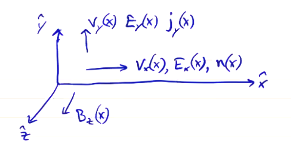
Physically, this means that waves can propagate, but only in the \( \vu x \) direction. To compute the fields from grid sources, we need to solve the full Maxwell’s equations. We’ll do so in Heaviside-Lorentz units:
\[\pdv{\vec E}{t} = c \curl \vec B - \vec j\] \[\pdv{\vec B}{t} = - c \curl \vec E\]
In the 1D-2V system, these become
\[\pdv{E_y}{t} = - c \pdv{B_z}{x} - j_y\] \[\pdv{B_z}{t} = - c \pdv{E_y}{x}\]
Let’s define some new variables:
\[F^+ \equiv \frac{E_y + B_z}{2}\] \[F^{-} \equiv \frac{E_y - B_z}{2}\]
These mean that
\[E_y = F^+ + F^-\] \[B_z = F^+ - F^-\]
So Maxwell’s equations become (in matrix form)
\[\pdv{}{t} \begin{bmatrix} F^+ \\ F^- \end{bmatrix} + c \pdv{}{x} \begin{bmatrix} F^+ \\ - F^- \end{bmatrix} = - \frac{1}{2} \vec j_y \begin{bmatrix} 1 \\ 1 \end{bmatrix}\]We notice the form of a conservation law. Notice on the left-hand side, we have the total derivative in Lagrangian frame moving at velocity \( \pm c \). We can define some other relevant terms. The Poynting flux is then
\[P = c \left[ \overbrace{(F^+)^2}^{\text{+ direction}} - \overbrace{(F^-)^2}^{\text{- direction}} \right]\]The energy density is \( (F^+)^2 + (F^-)^2 \). We can update the fields in the Lagrangian frame of reference
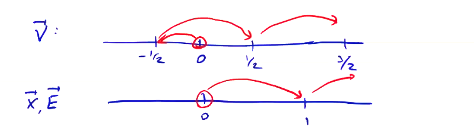
\[\frac{F^+( t + \Delta t, x + c \Delta t) - F^+(t, x)}{\Delta t} = - \frac{1}{2} j_y (t + \frac{\Delta t}{2}, x + c \frac{\Delta t}{2})\] \[\frac{F^-( t + \Delta t, x - c \Delta t) - F^-(t, x)}{\Delta t} = - \frac{1}{2} j_y (t + \frac{\Delta t}{2}, x - c \frac{\Delta t}{2})\]To properly center the current density relative to \( \vec E \), \( \vec B \) it must be centered at time step \( n + 1/2 \). Velocity is already centered properly to give \( j_y ^{n + 1/2} \). The location is given at \( x_i ^n \) and \( x_{i} ^{n+1} \), and are used to center \( j_y \) to the grid.
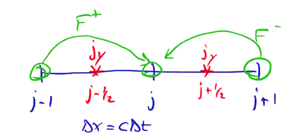
Considering the special case \( \Delta x = c \Delta t \), the method simplifies (though this is not a limitation of the method, just a simplified case):
\[{F_j^+}^{n+1} = {F_{j-1} ^+}^n - \frac{\Delta t}{4} \underbrace{\left({j_y}_j ^{n + 1/2} + {j_y}_{j - 1} ^{n + 1/2} \right)}_{2{j_y}_{j - 1/2}}\] \[{F_j^-}^{n+1} = {F_{j+1} ^-}^n - \frac{\Delta t}{4} \underbrace{\left({j_y}_j ^{n + 1/2} + {j_y}_{j + 1} ^{n + 1/2} \right)}_{2{j_y}_{j + 1/2}}\]
Current Weighting#
For arbitrary values of \( \Delta x \), we interpolate the value of \( j_y \) using the shape functions. Current weighting is always required for electrodynamic PIC. We still need charge weighting to compute \( E_x \).
Given the particle’s position at \( x_i ^n \) and \( x_i ^{n+1} \), we use the shape function to distribute \( v_i ^{n + 1/2} \) across \( j_{j - 1/2} ^{n + 1/2} \) and \( j_{j + 1/2} ^{n + 1/2} \)
\[{j_y}_{j \pm 1/2} ^{n + 1/2} = \sum_i q_i v_i ^{n + 1/2} \left[ \frac{S(x_{j \pm 1} - x_i ^{n + 1}) + S(x_j - x_i ^n)}{2} \right]\]Longitudinal Electric Field#
In electrodynamic PIC, the longitudinal electric field \( E_x \) is computed as we did in the electrostatic case
\[\div \vec E = \div ( E_x \vu x + E_y \vu y) = \pdv{}{x} E_x = \rho / \epsilon_0\]This implies that the wave vector \( \vec k \) is only in the \( \vu x \) direction.
Electrodynamic PIC algorithm#
To advance electrodynamic PIC by a single time step.
At time \( n-1 \), we already know:
- \( x^{n-1} \)
- \( v^{n-3/2} \)
- \( E_x ^{n-1} \)
- \( E_y ^{n-1} \)
- \( B_z ^{n-1} \)
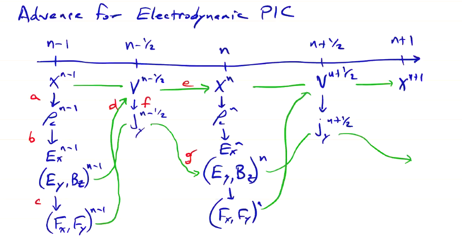
- At position \( x^{n-1} \), we compute the particle position \[x^{n-1} \rightarrow \rho_c ^{n-1}\]
- We solve Poisson’s equation using the source terms at \( n-1 \) \[\rho_c ^{n-1} \rightarrow E_x ^{n-1}\]
- Weight the fields to the grid to get forces \[E_x ^{n-1}, E_y ^{n-1}, B_z ^{n-1} \rightarrow F_x ^{n-1}, F_y ^{n-1}\]
- Advance the velocities using the weighted forces \[v^{n-3/2}, F_x ^{n-1}, F_y ^{n-1} \rightarrow v^{n-1/2}, j_y ^{n-1/2}\]
- Advance the particle’s position using the accelerated velocity \[v^{n-1/2} \rightarrow x^n\]
- Solve Maxwell’s equation to advance the transverse fields \[E_y ^{n-1}, B_z ^{n-1}, j_y ^{n-1/2} \rightarrow E_y ^n, B_z ^n\]
Application of PIC - Two Stream Instability#
An early use of the PIC method was investigation of beam-beam fusion. The idea is that you could quite easily achieve fusion by colliding two cold, counter-streaming beams. Two ion beams at 100keV can fuse to produce 17.6 MeV, at a gain of about 200. Easy peasy, right? It turns out the two-stream instability prevents us from achieving this exact scenario.
Initially, we can start with two cold beams. Uniform beams will exert no force on each other. But very quickly, we will see out of phase bunching. Any non-uniformity in the density will cause a perturbation in the velocity, along with a matching perturbation in the other beam. These perturbations travel in opposite directions, producing forces that mix the beams and thermalize the plasma. This converts kinetic into thermal energy, spreading the energy across a broad range of velocity. This means that the only ions that still have enough energy to fuse are those out at the tails of the distribution, so the gain goes to pot.
Dispersion Relation#
The dispersion relation for a cold plasma is:
\[\frac{\omega_p ^2}{\omega ^2} = 1\]If the plasma has a uniform velocity, such that the plasma becomes a cold beam, then the frequency is Doppler shifted
\[\frac{\omega_p ^2}{(\omega - k v_0) ^2} = 1\]And if we have two cold beams, then
\[\frac{{\omega_p}_1 ^2}{(\omega - k v_1)^2} +\frac{{\omega_p}_2 ^2}{(\omega - k v_2)^2} = 1\]For identical, counter-streaming beams, \( v_1 = - v_2 = v_0 \):
\[\frac{\omega_p ^2}{(\omega - k v_0)^2} + \frac{\omega_p ^2}{(\omega + k v_0)^2} = 1\]We can solve for \( \omega \) and plot \( |\omega| / \omega_p \) vs \( k v_0 / \omega_p \):
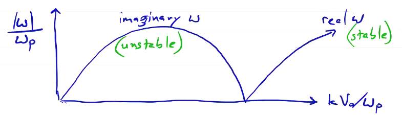
The unstable range where we have imaginary solutions for \( \omega \) is the two-stream instability. We got here from a linear analysis, so we assume \( v_1 \propto e^{-i \omega t} \). That’s why the unstable solution goes like \( e^{\gamma t} \). The dispersion relation is a linear result. As the instability grows over time, nonlinear effects (like trapped particles) and saturation determine the long-term solution.
Boundary Conditions for Finite Systems#
As with all PDEs, boundary conditions can critically affect the solution and require special numerical treatment. Let’s consider some specific boundary conditions.
- Conducting Wall. The wall will reflect EM fields: \[\vu n \cross \vec E = 0 \qquad \rightarrow \qquad \vec E_{\parallel} = 0\]
Gauss’s law tells us this leads to to the accumulation of a surface charge density
\[\vu n \cdot \vec E = \rho / \epsilon_0\] \[\rightarrow \vec E_n = \rho_s / \epsilon_0\] where \( \rho_s \) is a surface charge density.
\[\vu n \cdot \vec B = 0 \qquad \rightarrow \qquad \vec B_n = 0\] \[\vu n \cdot \pdv{\vec B}{t} = 0 \rightarrow \vec B_n = \text{const.}\] \[\vu n \cross \vec B = \mu_0 \vec j_s \rightarrow \vec B_t = \mu_0 \vec j_s \cross \vu n\] where \( \vec j_x \) is the surface current density.
- Insulating Wall. The boundary conditions for an insulating wall will depend on the dielectric properties of the insulating wall. For a perfect insulator,
\[\pdv{\vec E}{\vu n} = 0 \quad (\rho_s = 0)\] and \[\pdv{\vec B}{\vu n} = 0 \quad (\vec j_s \cdot \vu n = 0)\]
So that’s the fields taken care of. What about the particles? At a boundary, they can be reflected, absorbed, or emitted, depending on the material properties and the properties of the impacting/emitted particles. What happens when a particle hits a material boundary depends on:
- The work function of the material
- Secondary electron and ion emission coefficient
- Applied or induced field/potential
- Dielectric strength of material
- Sputtering properties
It is important to implement numerical boundary conditions that are consistent with the physics we’re trying to model.
Implementation - Reflected Particles#
For the reflection boundary condition, we want to generate a mirror image of the particle’s trajectory. To view the scenario, let’s look at a 1-dimensional particle traveling towards a reflecting boundary at \( x=0 \). We’ll plot position along the horizontal axis and time along the vertical.
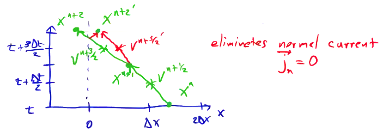
We reflect the velocity when the particle crosses the boundary, such that \( {v^{n + 3/2}}’ \) now takes us to the reflected position \( {x^{n + 2}}’ \) instead of \( x ^{n+2} \). This eliminates the normal current, \( \vec j _n = 0 \)
Implementation - Absorbed/Emitted particles#
For an absorption boundary, when charges and currents reach the boundary, they are deposited on the boundary and build up, unless it is an open boundary.
The inverse situation is emitting particles at the boundary. Charge and current from the boundary.
Let’s consider a configuration in which we have electrodes at both side of our boundary, with a driving external current \( I(t) \) flowing between them.
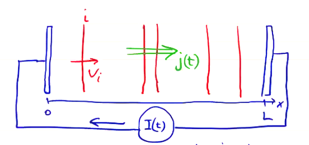
The total current \( I \) is the sum of hte convective plasma current and the displacement current. The total current density is
\[\vec j_{total} = (\rho \vec v)_{plasma} + \pdv{}{t} \vec E _{bias}\]where \( \vec E_{bias} \) is the electric field that will develop across the domain.
To fit such a boundary within our leapfrog framework, all of the values must be properly centered for computing Maxwell’s equations.
\[\vec j _{total} ^{n + 1/2} = \vec j _{plasma} ^{n + 1/2} + \frac{\vec E _{bias} ^{n+1} - \vec E _{bias} ^n}{\Delta t}\]where
\[\vec j_{plasma} ^{n + 1/2} = \frac{1}{L} \sum _i q_i \vec v_i ^{n + 1/2}\]and
\[\vec E_{bias} ^n = - \frac{\phi _b ^n - \phi _a ^n}{L} \vu x\]The current density is then used to solve Ampere’s law for the local electric field at the boundary \( \vec E_{local} \).
Particles are emitted from the electrode when the total electric field exceeds the threshold to pull particles from the surface (the work function). The process of pulling particles from the electrode when the field exceeds the work function is called field emission.
\[\vec E_{total} = \vec E_{bias} + \vec E_{local}\]We typically emit particles at \( x_j = \pm \Delta x / 2 \) with a Maxwellian distribution at the wall temperature using Monte Carlo. We emit particles as long as the fied exceeds the work function.
Absorption leads to material interactions. Absorbed particles deposit their energy into the surface. This can lead to effects like:
- secondary electron and ion emission
- sputtering
- surface heating, which can lead to thermionic emission
Implementation - Open Boundaries#
In general, open boundaries can be difficult for PIC and Poisson solvers in general. This can be thought of as an impedance mismatch between the domain and the boundary. This scenario might occur when we’re modeling plasmas in space, where we would like the boundary to be a perfect vacuum, and particles have no interaction with the boundary whatsoever. But with any impedance mismatch, we will get artificial reflections in the EM fields.
A common treatment for PIC codes is to append a dissipative layer to damp outgoing EM waves that enter the layer. Schematically, we draw this as a ramp-up of the impedance at the boundary over a width \( \delta \).
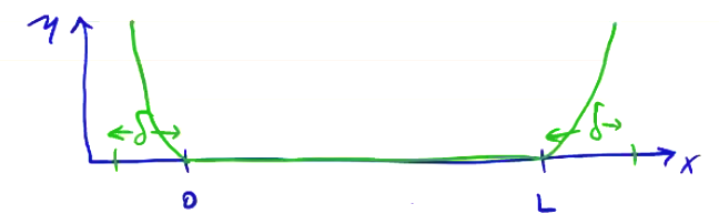
A damping layer like this which dissipates all EM fields is called a Perfectly Matched Layer (PML). To get a PML, \( \delta \) must be greater than the longest wavelength of fields in the system \( \lambda_{longest} \), or allow non-physical configurations \( \div \vec B = 0 \).