Multidimensional Electrodynamic PIC #

Now that we’ve touched on each of the components of a 1-dimensional electrodynamic PIC method, let’s try to move our model into a full multidimensional one. The main difficulty in moving from 1D to 2D/3D is the increased variety of waves present in the solution.

Field Equations #

The EM fields must be solved for the full Maxwell’s equations, not just Poisson’s equation, in order to capture the full dynamics.

Again, we’ll use our leapfrog algorithm to advance in time, with \( \vec j \) determined by the particle velocities, \( \vec v_i \) at \( n + 1/2 \).

We need to know the magnetic field at a different time step than the particle positions / electric field, so we’ll have to keep that in mind.

When we compute spatial derivatives like \( \curl \vec A \), they must also be centered. In 2D the curl is

In a naive implementation, we could simply calculate these spatial derivatives using finite differences placed at the cell vertices. This would give us estimates of the derivatives at the midpoints between the cells. But we need those derivatives at the cell vertices to determine \( \vec E \) and \( \vec B \), so we would have to perform some averaging. This means that splitting the curl operator to different locations reduces overall accuracy.

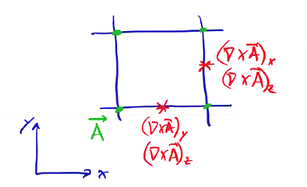
A much better approach is to not collocate the field components. Instead we use a “staggered grid” called a Yee grid.

• Store \( E_z \) at the grid points
• Store \( B_z \) at the center of the grid cell
• Store \( E_x \) and \( B_y \) along the horizontal
• Store \( E_y \) and \( B_x \) along the vertical cell edges

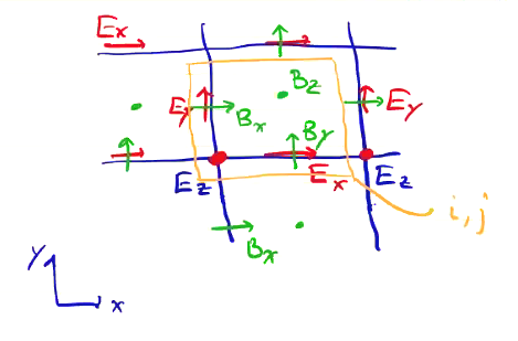
Differences on this staggered grid provide 2nd order accuracy for spatial derivatives, in a very similar way to the 2nd order accuracy we get from our leapfrog integration.

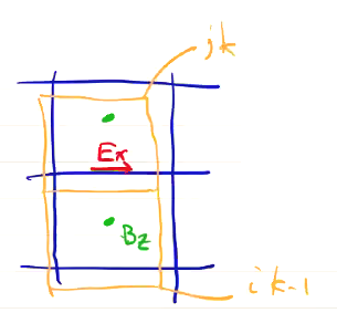
Let’s start with a differencing of Faraday’s law. We’re taking the difference \( E_x \) in the \( y \) direction, and the difference \( E_y \) in the \( x \) direction

Now let’s try Ampere’s law:

Here, we need the \( \vec j \) components to be collocated with the electric field \( \vec E \).

We only get second order accuracy from the Yee grid if \( \Delta x \) and \( \Delta y \) are constant, that is, if we have a uniform grid. Computing the spatial derivatives with mismatched cell sizes does not give second order accuracy. As we’ve written this, we don’t necessarily require \( \Delta x = \Delta y \), but we will require \( \Delta x = \Delta y \) later as we move particles through the grid.

The requirement \( \Delta x = \Delta y = const. \) means curved boundaries are difficult. Curved sections of boundaries must be stair-stepped:

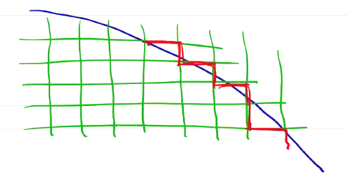
Resolving geometric details and features requires decreasing \( \Delta x, \Delta y, \Delta z \) globally. This is still an outstanding issue for PIC models. There has been some success with “cut cell” methods, in which the cells at the boundary are cut into triangles and trapezoids to match the curve of the boundary (with straight lines). This does solve the problem of resolving geometric detail at the boundary, but it means that those cells at the edge need to be treated differently from all of the other cells in the model. It’s also not entirely clear that cut cell methods preserve the second-order accuracy of Yee grids.

Particle Push #

For the particle advance, we want to advance velocities \( v ^{n - 1/2} \) to \( v^{n + 1/2} \), so the force is needed at time \( n \). This is fine for the electric field, which is known at \( n \). However, \( \vec B \) is known at \( n + 1/2 \). Again, we use Strang splitting to split the magnetic field advance into two stages. The initial advance gives us \( \vec B^n \):

After the particle push, advance \( \vec B \) again

This is a pretty trivial Strang splitting, just equivalent to an average \( \vec B^n = \frac{B^{n + 1/2} + B^{n - 1/2}}{2} \). That’s because Strang splitting is only really important when the quantity used to advance changes between the split advances.

Current Weighting #

Let’s talk about how to perform current weighting. We need to weight the particles’ trajectories at the grid points. We’ll do this in the same manner as in 1D. Here are a couple of options.

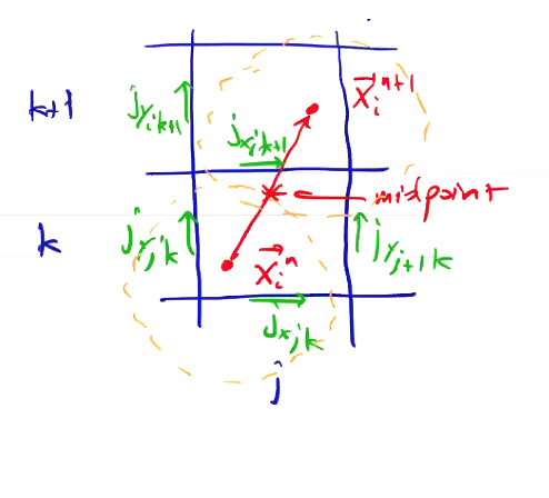
• Method 1: \[\vec j_{j, k} ^{n + 1/2} = \sum _i q_i \vec v_i ^{n + 1/2} \left[ \frac{ S(\vec x_{j, k} - \vec x _i ^{n + 1}) + S(\vec x _{j, k} - \vec x ^n)}{2} \right]\]

• Method 2: Use the midpoint position \( \vec x_i ^{n + 1/2} = \frac{1}{2} (\vec x_i ^{n + 1} + \vec x_i ^n) \), so we use the shape function at \[S(\vec x_{j, k} - \vec x_i ^{n + 1/2})\]

Depending on the location we use for the shape function, we will get different results. Consider an example case of particles moving from \( \vec x_i ^n \) to \( \vec x_i ^{n+1} \):

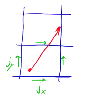
Let’s try out Method 1, using nearest grid point weighting with the above particle positions:

For nearest grid point, we just check which grid element is inside the particle extent for particle \( \vec x_i \).

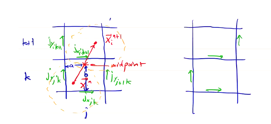
For method 2, let \( b \) be the vertical distance from cell \( i, j \) to the midpoint \( \vec x_i ^{n + 1/2} \), and \( a \) be the horizontal distance from cell \( i, j \) to the midpoint \( \vec x_i ^{n + 1/2} \).

\[{j^{n + 1/2}_x}_{j, k} = \frac{1 - b}{\Delta x} q_i {v_x ^{n + 1/2}}_i\] \[{j^{n + 1/2}_x}_{j, k+1} = \frac{b}{\Delta x} q_i {v_x ^{n + 1/2}}_i\] \[{j^{n + 1/2}_y}_{j, k} = \frac{1 - a}{\Delta y} q_i {v_y ^{n + 1/2}}_i\] \[{j^{n + 1/2}_y}_{j+1, k} = \frac{a}{\Delta y} q_i {v_y ^{n + 1/2}}_i\]

We see that the different weighting methods give different current distributions. As it turns out, method 1 is better at conserving charge. Methods exist that exactly conserve charge by satisfying Poisson’s equation. Villasenor & Bunemen (Comp Phys. Comm. 69 306, 1992) is such a method, and is the standard method used for PIC methods.

We can see the connection between charge conservation and current weighting by looking at Poisson’s equation

\[q_\alpha \left( \pdv{n_\alpha}{t} + \div (n_\alpha \vec v_\alpha) \right) = 0\] \[\pdv{}{t} \left( q_i n_i - e n_e \right) + \div (q_i n_i \vec v_i - e n_e \vec v_e) = 0\] \[\pdv{\rho_c}{t} + \div \vec j = 0\] \[\div \vec j = - \pdv{}{t} (\rho) = \pdv{}{t} (\epsilon_0 \grad ^2 \phi)\]

The reason our two methods don’t do a very good job at charge conservation is that they do not preserve the correct value of \( \div \vec j \).

In multi-dimensional EM PIC, we no longer have to weight charges to the grid, because we no longer need to solve Poisson’s equation. The only equations we need are Faraday and Ampere.

Particle Advance #

Advancing particles requires weighting the fields at the particle locations

\[\frac{\vec v_i ^{n + 1/2} - \vec v_i ^{n - 1/2}}{\Delta t} = \frac{ \vec F_i ^n}{m_i}\] \[\frac{\vec x_i ^{n + 1} - \vec x_i ^n}{\Delta t} = \vec v _i ^{n + 1/2}\]

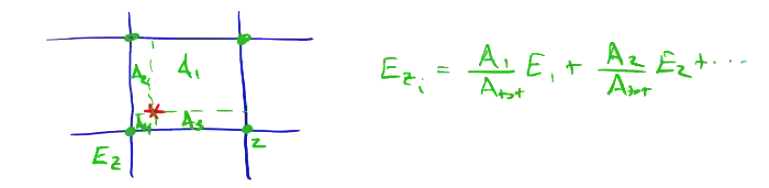
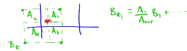
Forces are weighted to particle positions using 1st-order particle shape, which amounts to using inverse areas for each sub-grid for the various field components. For example, the electric field is weighted to the nearest grid points by the inverse areas as shown:

The magnetic field will be weighted to the nearest half-grid points (cell centers)

Only the time-dependent Maxwell’s equations are evolved to advance \( \vec E \) and \( \vec B \). We still the divergence constraints. Gauss’s law has to be initially satisfied; afterwards, mathematically they are preserved.

\[\div \vec B = 0\] \[\div \vec E = \rho / \epsilon_0\]

If we take the divergence of Faraday’s law, \[\pdv{}{t} \div \vec B + \div ( \curl \vec E) = 0 \rightarrow \pdv{}{t}(\div \vec B ) = 0\]

We can do the same with Ampere’s law \[\pdv{\vec E}{t} = \frac{1}{\epsilon_0} \vec j = c^2 \curl \vec B\] \[\pdv{}{t}( \div \vec E) + \frac{1}{\epsilon_0} \div \vec j = c^2 \div ( \curl \vec B) \\ \rightarrow \pdv{}{t} \left(\div \vec E - \frac{1}{\epsilon_0} \pdv{\rho}{t} \right) = 0\]

So if Gauss’s law is initially satisfied, then it will remain so over time. Divergence cleaning techniques are sometimes used to help maintain.

In practice, Poisson’s equation is solved for the initial particle locations and applied fields, throughout the domain. This gives \( \vec E(t = 0) \). The Biot-Savart law is solved for the initial internal currents and applied magnetic fields, giving \( \vec B (t = 0) \). With these initial fields, we then only advance using Faraday and Ampere.

As an example, consider a Penning trap, consisting of a solenoidal coil (which applies external magnetic field \( B_ext \)) and a circumferential electrode held at potential \( \phi_3 \) with respect to end electrodes \( \phi_1 = \phi_2 \).

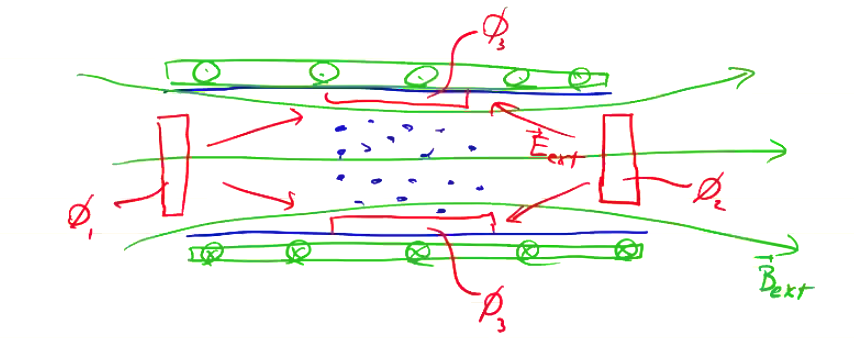
With \( \phi_1 > \phi_3 \), positively charged particles will be trapped in the center of the configuration, gyrating about the magnetic field. When modeling a Penning trap, we initially need to solve for the fields due to both the initial particle distribution and the electrodes, and the magnetic field due to both the particles and the externally applied field.