Fluid Models for Plasmas #

Motivation for Fluid Models #

Up to this point, we’ve been discussing particle models, and in particular, kinetic descriptions in which we’ve sampled the distribution function at particular locations to get our particles. We retained detailed information about the distribution function by tracking the positions and velocities of these representative super-particles, which should continue to “represent” the sampled distribution function at all points in time. Tracking this detailed information is computationally expensive, so PIC is limited to small spatial scale or short time scale phenomena. Non-linear waves and wave-plasma interactions are good examples of PIC use cases.

Applying 3D kinetic models to a confined plasma, for example, stretches beyond the current state of the art. This desire motivates the use of reduced models. Fluid models are examples of reduced models.

Other courses (like the course under the “MHD Theory” section of these notes) go into much more detail on fluid models, so this section will not be as complete as the PIC description.

Moment Reductions #

Fluid models reduce the information about the distribution functions, retaining only the minimum required information to characterize the distribution. This is done by retaining velocity moments of \( f(\vec v) \).

• 0th moment \( \int f(v) \dd v \) is the number density
• 1st moment \( \int v f(v) \dd v \) gives the mean particle velocity, also called the drift or fluid velocity.
• 2nd moment \( \int (v - v_d)(v - v_d) f(v) \dd v \) gives the root mean square of the particle velocity, related to the fluid temperature.

These three moments are the only ones required to describe a Maxwellian distribution. A fluid system which tracks only these three moments necessarily assumes a local thermodynamic equilibrium (LTE). We don’t have to assume LTE; we can allow for deviations away from a Maxwellian distribution, but we must include additional moments to do so.

• 3rd moment (skewness) is related to the energy flux.
• 4th moment (kurtosis) doesn’t have a precise physical meaning, referred to as the “weight of the tail of the distribution.”

The higher moments are really just statistical concepts, without real physical meaning.

Fluid models evolve only the moments of \( f( \vec v) \) to reduce the dimensionality of a full 6D (3P-3D) kinetic description down to a three-dimensional description

We’ve gone back down from 6D to 3D, but we have more variables at each point (moment values are scalars, vectors, and even tensors).

Moments for species \( \alpha \) are defined as

where \( \vec v^{n} \) is the vector dyad product of \( \vec v \) with itself. This means that in general, \( {M_{\alpha}}_{n} \) will be a tensor, for each species \( \alpha \) in our system. These are the primary dependent variables of the fluid model.

\[n = 0: \qquad \int f_{\alpha} \dd \vec v = n_{\alpha}\] \[n = 1: \qquad \frac{\int \vec v f_{\alpha} \dd \vec v}{n_{\alpha}} = \vec v_{\alpha}\] \[n = 2: \qquad \int m_{\alpha} ( \vec v - \vec v_{\alpha})( \vec v - \vec v_{\alpha}) f_{\alpha} \dd \vec v = \overline{\vec P_{\alpha}}\] \[n = 3: \qquad \frac{1}{n_{\alpha}} \int m_{\alpha} (\vec v - \vec v_{\alpha})(\vec v - \vec v_{\alpha}) ( \vec v - \vec v_{\alpha}) f_{\alpha} \dd \vec v = \overline{\vec H_{\alpha}}\]

where \( n_{\alpha} \) is a rank 0 tensor, \( \vec v_{\alpha} \) is a rank 1 tensor, \( \overline{ \vec P}{\alpha} \) is a rank 2 tensor (with only 6 unique components), \( \overline{\vec H}{\alpha} \) is a rank 3 tensor, and so on.

A common reduction is to define a heat flux vector (tensor contraction) \[\vec h_{\alpha} = \frac{m_{\alpha}}{n_{\alpha}} \int ( \vec v - \vec v_{\alpha}) \cdot ( \vec v - \vec v_{\alpha})(\vec v - \vec v_{\alpha}) f_{\alpha} \dd \vec v\] by contracting a dimension, we get a vector, which is the standard heat flux vector we usually think about. The full system is the 13N-moment plasma model (where N is the number of species). The moments are: \( n \), \( v_x \), \( v_y \), \( v_z \), \( P_{xx} \), \( P_{xy} \), \( P_{xz} \), \( P_{yy} \), \( P_{yz} \), \( P_{zz} \), \( h_z \), \( h_y \), \( h_z \) for each species \( \alpha \).

To cap off the moments, we need to “close” the model with a closure expression. Typically, we define a closure for the heat flux by defining a Fourier law for the conductivity:

This is the 10N-moment plasma model.

5N-Moment Model #

Another reduction is to define a closure for the anisotropic pressure tensor. This leaves us with the isotropic pressure (and temperature), and the shear stress is related to lower moment variables by a viscosity, like \( \nu \grad \vec v \). We then end up with the 5N-moment plasma model, which is one of the most common models for capturing many fluids. It’s typically called the multi-fluid plasma model.

The governing equations are derived by taking moments of the Boltzmann equation

\[n = 0: \quad \pdv{n_{\alpha}}{t} + \div ( n_{\alpha} \vec v_{\alpha}) = 0\] \[n =1: \quad n_{\alpha} m_{\alpha} \left( \pdv{\vec v_{\alpha}}{t} + \vec v_{\alpha} \cdot \grad \vec v _{\alpha} \right) + \div \overline{\vec P}_{\alpha} - n_{\alpha} q_{\alpha} ( \vec E + \vec v_{\alpha} \cross \vec B) \\ = m_{\alpha} \int \vec v \left. \pdv{f_{\alpha}}{t} \right| _{coll} \dd \vec v \\ = - \sum_ \beta n_{\alpha} m_{\alpha} ( \vec v_{\alpha} - \vec v_\beta) \nu_{\alpha \beta} = \sum_\beta - \vec R_{\alpha \beta}\]

Note that this is the full Boltzmann equation, not the Vlasov equation, so we include the collision operator \( \vec R_{\alpha \beta} \) between unlike species \( \alpha \) and \( \beta \).

\[\overline{\vec P}_{\alpha} = P_{\alpha} \overline{\vec I} + \overline{\vec \Pi}_{\alpha}\] where the scalar pressure is \( P_{\alpha} = n_{\alpha} k T_{\alpha} \)

where \( \dot{Q} _ {\alpha} \) includes the thermal conduction (heat flux vector), collisional heating (Ohmic heating), radiation losses, external heating, and so on. In this way, we’ve used our equations of state (closures) to express the full equations of motion in terms of our 5N moments \( (n, \vec v, T) _ {\alpha} \). The closure relations we’ve used for higher moment variables are \[\overline{\vec \Pi}_{\alpha} = \nu _{\alpha} \grad \vec v_{\alpha}\] \[\vec h_{\alpha} = - \kappa _{\alpha} \grad T_{\alpha}\] where the constants \( \nu_{\alpha} \) and \( \kappa_{\alpha} \) are called “transport coefficients.” They represent any physics which are not accurately captured by the LTE system, and so they represent approximations.

Equations of State #

Equations of state are used in defining closure relations. For example, for isothermal conditions, \( T_{\alpha} \) is constant, so \( P_{\alpha} \propto n_{\alpha} \).

Another assumption might be a force-free, cold assumption, so \( T_{\alpha} = 0 \) and therefore \( P_{\alpha} = 0 \).

Adiabatic assumption gives \( P_{\alpha} \propto n_{\alpha} ^\gamma \) for adiabatic index \( \gamma \) (ratio of specific heats).

Equations of Motion #

The fields are governed by Maxwell’s equations

\[\epsilon_0 \div \vec E = \sum _\alpha q_\alpha n_\alpha\] \[\div \vec B = 0\] \[\epsilon_0 \pdv{\vec E}{t} = \frac{1}{\mu_0} \curl \vec B - \sum_\alpha q_\alpha n_\alpha \vec v _\alpha\] \[\pdv{\vec B}{t} = - \curl \vec E\]

The thermal conductivity \( \vec \kappa \) and electrical resistivity \( \vec \eta \) are often functions of the magnetic field \( \vec B \).

Single-Fluid MHD Model #

To reduce the 5N fluid model even further, we work to combine the ions and electrons into a single fluid by applying some asymptotic approximations.

\[\epsilon_0 \rightarrow 0 (c \rightarrow \infty) \quad \text{and} \quad m_e \rightarrow 0\] \[n_e = Z n_i = n \quad \text{Quasineutrality}\] \[Z = 1, q = e \quad \text{Singly-charged}\]

We define our MHD variables as the center-of-mass values:

The mass density \( \rho \) is approximately the ion density

The center-of-mass velocity is approximately the ion velocity

The pressure is the sum of the species pressures

And the current density is approximately the electron current density

We now write the MHD equations in terms of the center of mass quantities

Continuity:

Momentum:

We’ll want to revisit the negligible electron mass approximation. If we neglect the electron mass, then the \( m_e \vec v_e \cdot \grad \vec v_e \) term can not necessarily be dropped. However, if we neglect the electron inertia, then we can drop it. Doing so gives

The generalized Ohm’s law relates current density to the electric field

For \( m_e \ll m_i \) and \( m_e v_e \ll m_i v_i \), we get the single-fluid equation of motion:

Assumptions / Asymptotic Approximations #

Let’s be specific about our assumptions, and provide justifications.

The negligible electron mass \( m_e \ll m_i \) is okay since \[\frac{m_e}{m_i} < \frac{1}{1836} \approx 0.05 \%\]

Quasineutrality \( n_i = n_e \) is accurate down to some scale. If we have a globally neutral plasma \( N_i = N_e \), then scale is the Debye length \( L \gg \lambda_D \).

The negligible electron inertia \( m_e v_e \ll m_i v_i \) is not always justified

\[j = n e (v_i - v_e) = n e v_i \left( 1 - \frac{v_e}{v_i} \right)\] \[\frac{m_e v_e}{m_i v_i} = \frac{m_e}{m_i} \left( 1 - \frac{1}{M} \frac{j}{n e v_{th}} \right)\]

where the Mach number \( M \) is \( v_i / v_{th} \).

Let’s see how well this approximation checks out in a laboratory plasma. In the ZaP experiment,

\[I = 10^5A \qquad n = 10^{22} m^{-3} \qquad v_{th} = 10^5 m/s\] \[M = 1 \qquad a = 0.01m\] Plugging everything in, we get \[\frac{m_e v_e}{m_i v_i} = 0.3\%\]

So, not a bad assumption. In contrast, in the HIT-SI3 experiment, we have

\[I = 10^4 \qquad n = 10^{19} m^{-3} \qquad v_{th} = 10^4 m/s \\ M = 0.1 \qquad a = 0.1 m\] In this case, \[\frac{m_e v_e}{m_i v_i} = 10\%\] so the single-fluid approximation does not necessarily apply well there. We might think that moving to larger and larger scale lengths inevitably breaks this assumption, but in a really big tokamak (ITER) we do a pretty good job

\[I = 10^6 A \qquad n = 10^{20} m^{-3} \qquad v_{th} = 10^6 m/s \\ M =0.1 \qquad a = 1 m\] \[\frac{m_e v_e}{m_i v_i} = 0.2 \%\]

Ultimately, most of our assumptions boil down to a low frequency assumption, since large spatial scales and slow evolution, such that \( c \rightarrow \infty \) imply low frequency evolution, and the quasineutral condition \( L \gg \lambda_D \) leads to a large frequency \( \omega_p = v_{th} / \lambda_D \). For \( \omega \ll \omega_p \), we can drop the left-hand side of the generalized Ohm’s law

For quasineutrality, we can also drop the displacement current from Ampere’s law

\[\mu_0 \epsilon_0 \pdv{\vec E}{t} \approx 0 = \curl \vec B - \mu_0 \vec j\] \[c^2 \rightarrow \infty, \quad \mu_0 \epsilon_0 = 1/c^2 \rightarrow 0\] \[\epsilon_0 \div \vec E = \rho_c \rightarrow 0\]

Taken together, this is the Hall-MHD plasma model, which is the most complete single-fluid MHD model available.

If the Hall and diamagnetic terms are negligible, we have well magnetized ions with small Larmor radius \( r_{L, i} \):

then the generalized Ohm’s law becomes

This is the Resistive MHD model. If we remove collisions entirely (\( \eta \rightarrow 0 \)), then we have the Ideal MHD Model.

The energy equation is still:

If we use the definition of energy

If we take the time derivative of this,

To get the second term, it helps to dot \( \vec v \) with \( v \):

and similarly, taking the dot product of \( \vec B \) with the induction equation helps to get the third term

For all of these assumptions, the single-fluid MHD model is widely applicable to many plasmas.

Numerical Solution of Fluid Models #

The equations of the plasma fluid models result in different characteristics of the dynamics, depending on the model and the physics that are captured by that model. We can get an idea of what those characteristics are by analyzing the governing equation type, which dictates the appropriate numerical algorithm.

Equation Types #

In general, PDEs and systems of PDEs can be classified as elliptic, parabolic, or hyperbolic.

Consider a general second-order ordinary scalar PDE given by

The canonical equation for this PDE in canonical form is

The PDE is

• elliptic if \( b ^2 < 4 a c \)
• paraboolic if \( b^2 = 4 a c \)
• hyperbolic if \( b^2 > 4 a c \)

For example, Poisson’s equation is an elliptic equation

\[\pdv{^2 \phi}{x^2} + \pdv{^2 \phi}{y^2} = - \rho / \epsilon_0\] \[b = 0 \quad 4ac = 4 \rightarrow b^2 - 4 a c < 0\]

The equation for magnetic diffusion is a parabolic equation

\[\pdv{B_z}{t} = \frac{\eta}{\mu_0} \pdv{^2 B_z}{x^2}\] \[b = 0 \quad 4 a c = 0 \rightarrow b^2 - 4 ac = 0\]

Maxwell’s equations in a vacuum are hyperbolic:

\[\pdv{\vec E}{t} = c \curl \vec B\] \[\pdv{\vec B}{t} = - c \curl \vec E\] \[\pdv{^2 \vec B}{t^2} = - c \curl \left( \pdv{\vec E}{t} \right) = c^2 \nabla ^2 \vec B\]

In 1D, \[\pdv{^2 B_z}{t^2} = c^2 \pdv{^2 B_z}{x^2}\] \[b = 0 \quad 4 a c = - 4 c^2 \rightarrow b^2 - 4 a c > 0\]

Hyperbolic Equations #

For hyperbolic PDEs, the solution at any point depends on a subset of the domain (domain of dependence), and it influences a subset of the domain (domain of influence). This is the same concept as a light cone, where only portions of the domain less than \( \pm c t \) away from the current time can affect the current state.

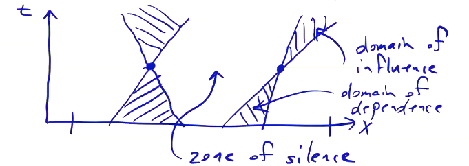
The slope of the curves that define the domains of influence/dependence are the characteristics of the equation. They are velocities; typically hyperbolic PDEs describe wave-like behavior, where the characteristic is the speed of the wave. The solution at a point does not necessarily depend on the boundary conditions; it will only do so when the domain of dependence intersects the boundary.

Parabolic Equations #

Parabolic PDEs have solutions that depend on the entire domain, but only at previous times. The domain of dependence includes the boundary conditions, and the initial condition.

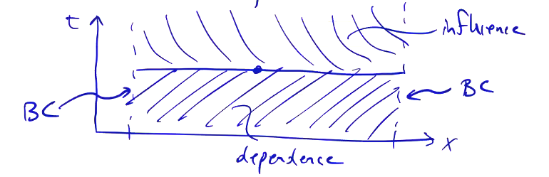
Parabolic PDEs are generally associated with diffusion-like behavior. The heat equation, viscous flow are parabolic equations.

Elliptic Equations #

For elliptic PDEs, the solution depends on and influences every other point in the domain. The boundary conditions and initial conditions determine the solution at every point in the domain.

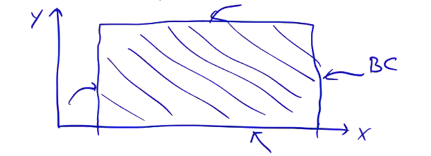
These equations are associated with steady-state and eigenvalue problems.

We’ve done this analysis assuming that the constants \( a \), \( b \), \( c \), … are just that, constant. If they depend on \( x \), \( y \), or the solution \( \psi \) itself, then the equation type can change.

Systems of Equations #

As we’ve written it, the MHD model is not a scalar equation, but rather a system of equations. To deal with systems of PDEs, we typically write the system as a vector equation in conservation form, then examine the eigenvalues:

where \( \vec Q \) is the vector of variables, and \( \vec F \) is the vector of fluxes. We can define the flux Jacobian \( \overline \vec A \equiv \pdv{\vec F}{\vec Q} \) and rewrite the governing system as an eigenvalue problem

The equation type is given by the characteristics of the flux Jacobian:

• Elliptic if the eigenvalues of \( \overline \vec A \) are imaginary.
• Parabolic if eigenvalues of \( \overline \vec A \) are repeated and the eigenvectors are not unique.
• Hyperbolic if the eigenvalues of \( \overline \vec A \) are real and the eigenvectors are unique.

Equation type of Ideal MHD Model #

Let’s apply this analysis to our ideal MHD model.

\[\pdv{\vec Q}{t} + \div \overline \vec T = 0\] where the vector of variables is

and the flux tensor is

Note that the vector of variables expands out to all of the various components of the vectors we’ve written:

We call a system of equations “conservative” if the time derivative of a conserved quantity can be written as a divergence of a flux. The divergence theorem makes this clear

Splitting \( \overline{\vec T} \) into components along the \( x \), \( y \), \( z \) directions,

where \[\vec F = \begin{bmatrix} \rho u \\ \rho u^2 - B_x ^2 / \mu_0 + p + B^2 / 2 \mu_0 \\ \rho u v - B_x B_y / \mu_0 \\ \rho u w - B_x B_z / \mu_0 \\ 0 \\ u B_y - B_x v \\ u B_z - B_x w \\ \left( e + p + \frac{B^2}{2 \mu_0} \right) u - \frac{\vec B \cdot \vec v}{\mu_0} B_x \end{bmatrix}\]

and similar for \( \vec G \), \( \vec H \). To determine the equation type of our system in 1 dimension, we want to calculate the eigenvalues of the flux Jacobian of \( \vec F \)

\[\pdv{\vec Q}{t} + \pdv{\vec F}{x} = 0\] \[\pdv{\vec Q}{t} + \underbrace{\pdv{\vec F}{\vec Q}}_{\vec A} \pdv{\vec Q}{x} = 0\] where \[\vec A = \begin{bmatrix} \left. \pdv{F_1}{Q_1} \right|_{Q_i} & \left. \pdv{F_1}{Q_2} \right|_{Q_i} & \ldots \\ \left. \pdv{F_2}{Q_1} \right|_{Q_i} & \ldots & \ldots \\ \ldots & \ldots & \ldots \end{bmatrix}\]

When we compute these derivatives, we need to be careful to keep our other conserved quantities constant. For example,

because \( (\rho u) \) is one of the conserved quantities. For \( F_2 \),

where we can write the pressure in terms of the conserved quantities as

\[p = (\gamma - 1) \left[ e - \frac{(\rho u )^2 + (\rho v)^2 + (\rho w)^2}{2 \rho} - \frac{B_x ^2 + B_y ^2 + B_z ^2}{2 \mu_0} \right]\] \[\pdv{p}{Q_1} = (\gamma - 1) \left[ \frac{(\rho u )^2 + (\rho v )^2 + (\rho w )^2}{2 \rho ^2} \right] = (\gamma - 1) \frac{u^2 + v^2 + w^2}{2}\] \[\pdv{F_2}{Q_2} = 2 \frac{(\rho u)}{\rho} + \pdv{p}{Q_2} = 2 (2 - \gamma) u\] \[\pdv{F_2}{Q_3} = \pdv{p}{Q_3} = 2(1 - \gamma) v\]

And so on and so forth for the other elements of \( \vec A \). Once we’ve got the flux Jacobian, we can compute the eigenvalues and eigenvectors of \( \vec A \). These will all be real-valued, which tells us that the ideal MHD equations are hyperbolic.

The Resistive MHD model can be written as

We know that \[\pdv{\vec Q}{t} + \frac{1}{R_m} \div \overline{\vec T_p} = 0\]

If we go through the same process for \( \overline{\vec T_p} \), we’ll find a parabolic system of equations, which is what we would expect from something with “resistive” in its name. So what sort of system is resistive MHD. The answer is, of course, “it depends.” Depending on the type of phenomena we expect to see in a particular configuration, we’ll have a dominant character associated with either wave phenomena or diffusive phenomena. The dominant character determines the appropriate algorithm to use when solving resistive MHD. For example, a large Reynolds number makes the system more hyperbolic.