Finite Difference Methods for MHD#
So for 1D MHD, we want to derive algorithms to advance the governing equations in time that have the form
\[\pdv{\vec Q}{t} + \pdv{\vec F}{x} = 0\]We can use the advection equation as a model equation: \[\pdv{u}{t} + a \pdv{u}{x} = 0\] which has the general solution \[u(x - at) = \text{const.} = u(x, t=0)\]
If we apply a forward Euler finite difference operators to our PDE,
\[\frac{u_j ^{n+1} - u^n _j}{\Delta t} + a \frac{u _{j+1} ^n - u_{j-1} ^n}{2 \Delta x} = 0\]Stability#
A brief von Neumann stability analysis shows that this forward Euler differencing is unstable. The way von Neumann stability analysis works, we assume a wave structure for the solution \[u_j ^n = A^n e^{i k x} = \underbrace{A ^n}_{\text{wave amplitude}} \cdot \overbrace{e^{i k j \Delta x}}^{\text{wave structure}}\]
If we substitute this form into our finite difference expression, we have
\[A^{n+1} e^{i k j \Delta x} = A^n e^{i k j \Delta x} - \frac{a \Delta t}{2 \Delta x}\left(A^n e^{i k (j+1) \Delta x} - A^n e^{i k (j-1) \Delta x} \right)\] We’re interested in the growth of the amplitude \( A^n \), called the amplification factor \( G \): \[G \equiv \frac{|A^{n+1}|}{|A^n|}\]
For forward Euler, we find \[\begin{aligned} \frac{A^{n+1}}{A^n} & = & 1 - \frac{a \Delta t}{2 \Delta x} \left( e^{i k \Delta x} - e^{- i k \Delta x} \right) \\ & = & 1 - \frac{i a \Delta t}{\Delta x} \sin (k \Delta x) \\ G & = & \sqrt{\left( \frac{A^{n+1}}{A^n} \right) \left( \frac{A^{n+1}}{A^n} \right)^\star} \\ & = & \sqrt{1 + \left( \frac{a \Delta t}{\Delta x}\right) ^2 \sin ^2 (k \Delta x)} \\ & \geq & 1 \quad \text{if} \quad \Delta t > 0 \end{aligned}\]
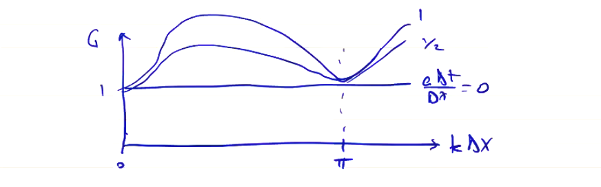
We find that the forward time, centered space (FTCS) algorithm is unconditionally unstable, for any values of \( k \), \( \Delta t > 0 \). Not a very good choice for solving the advection equation! However, the FTCS algorithm is an important component of many finite difference schemes which are stable.
Physically, the difficulty with the advection term can be seen in the continuity equation
\[\pdv{\rho}{t} + \vec v \cdot \grad \rho = - \rho \div \vec v = 0 \quad \text{(incompressible)}\]Using the FTCS difference approach to compute the gradients, we’re assuming that the gradient at node \( j \) is constant over the time interval \( n \rightarrow n + 1 \). This is only valid if the density profile is linear, and for non-linear profiles the gradient is inaccurate.

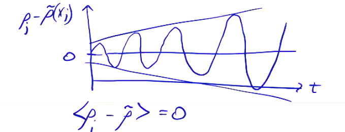
If we approximate the gradient of the density as
\[\pdv{\rho}{x} \approx \frac{\rho _{j+1} - \rho_{j - 1}}{2 \Delta x}\]then we get an error that is the difference between the line tangent at \( j - 1 \) and the line tangent at \( j \). We should actually calculate the gradient at \( t + \Delta t / 2 \) (assuming the flow is in the positive direction). The error leads to an over-estimate of the gradient magnitude, which leads to oscillations, which ultimately leads to instability.
Stable Solution Approaches for Advection Equation#
There are a few approaches we can take to come up with a finite differencing scheme which avoids this instability.
- Since the error is oscillating positive and negative, we can add diffusion to smooth out the error. This is the same as applying a time-average of the error to smooth the solution.
Spatial smoothing also works:
Noting that G increases with \( k \Delta x \), the shortest wavelengths grow the fastest, which is why a diffusive term helps smooth out the instability.
- Since the error is caused by computing the gradient at the wrong location, e.g. \( x_j \) instead of \( x_j - v \Delta t / 2 \), we can use upwind differencing
- Flux can be calculated as before, but we can apply limits to prevent minima or maxima from developing. Some approaches like this in the literature are
- total variation diminishing
- total variation bounded
- flux corrected transport
- Eliminate the advection term, or reduce it. If we write out the MHD equations in such a way that the advection term \( \vec v \cdot \grad \) is split out from the rest:
\[\pdv{\rho}{t} + \vec v \cdot \grad \rho = - \rho \div \vec v\] \[\pdv{\vec v}{t} + \vec v \cdot \grad \vec v = ( - \grad p + \vec j \cross \vec B) / \rho\] \[\pdv{\vec B}{t} + \vec v \cdot \grad \vec B = - \vec B \div \vec v + \vec B \cdot \grad \vec v\] \[\pdv{p}{t} + \vec v \cdot \grad p = - \Gamma p \div \vec v\]
If we let the grid move at the fluid velocity \( \vec v \)
\[\vec u _{grid} = \vec v\]then the advection term becomes
\[\vec v \cdot \grad \rightarrow ( \vec v - \vec u _{grid}) \cdot \grad\]which vanishes. Codes like this, expressing the equations of motion in Lagrangian frame of reference, are generally called ALE codes (Arbitrary Lagrangian Eulerian).
Method 1: Lax Algorithm#
To solve
\[\pdv{u}{t} + a \pdv{u}{t} = 0\]we had written the FTCS finite difference scheme:
\[u_j ^{n+1} = u_j ^n - \frac{a \Delta t}{2 \Delta x} \left( u_{j+1} ^n - u_{j-1} ^n \right)\]We can add diffusion by replacing \( u_j ^n \) with a local spatial average, giving us the Lax algorithm:
\[u_j ^n \rightarrow \frac{u_{j+1} ^n + u_{j - 1} ^n}{2} \quad \text{Lax Algorithm}\]If we apply the same von Neumann stability analysis as before, we find that
\[G = \sqrt{1 - \left[1 - \left(\frac{a \Delta t}{\Delta x}\right)^2 \right] \sin ^2 (k \Delta x)}\] So we have a stable solution if \[\left| \frac{a \Delta t}{\Delta x} \right| \leq 1 \quad \text{Courant condition}\]
This condition (also called the CFL condition) shows up quite a lot in fluid dynamics algorithms. It effectively limits the time step \[\Delta t \leq \Delta x / a\]
If we carry the substitution through our finite difference equation, we can see how the Lax method really does add a diffusion term:
\[u_j ^{n+1} = \underbrace{u_j ^n - \frac{a \Delta t}{2 \Delta x} (u_{j+1} ^n - u_{j - 1} ^n)}_{\text{FTCS}} + \underbrace{\left( \frac{u_{j+1} ^n - 2 u_j ^n + u_{j-1} ^n}{2} \right)}_{\text{Lax modification}}\]Manipulating the terms a bit,
\[\frac{u_j ^{n+1} - u_j ^n}{\Delta t} + a \left( \frac{u_{j+1} ^n - u_{j-1} ^n}{2 \Delta x} \right) = \frac{\Delta x^2}{2 \Delta t} \left( \frac{u_{j+1} ^n - 2 u_j ^n + u_{j-1} ^n}{\Delta x ^2} \right)\]which approximates the PDE
\[\underbrace{\pdv{u}{t} + a \pdv{u}{x}}_{\text{original PDE}} = \underbrace{\frac{\Delta x ^2}{2 \Delta t} \pdv{^2 u}{x^2}}_{\text{diffusion term}}\]In the limit of \( \Delta x \rightarrow 0 \) goes to zero, the diffusion term disappears and we recover the original PDE. It has the unfortunate property that the diffusion term grows as \( \Delta t \rightarrow 0 \), so we only retain accuracy as long as \( \Delta x ^2 \) goes to zero faster than \( \Delta t \).
Lax-Wendroff Algorithm#
Another algorithm known as the Lax-Wendroff algorithm can be less diffusive and is better behaved. It’s also derived from a more mathematically rigorous method than the Lax method. We get it through a process called a Cauchy-Kowalevskaya method.
We can derive Lax-Wendroff as a 2-step method:
- Use the Lax algorithm to advance the solution from \( t \) to \( t + \Delta t / 2 \)
- Use the leapfrog algorithm to advance from \( t \) to \( t + \Delta t \)
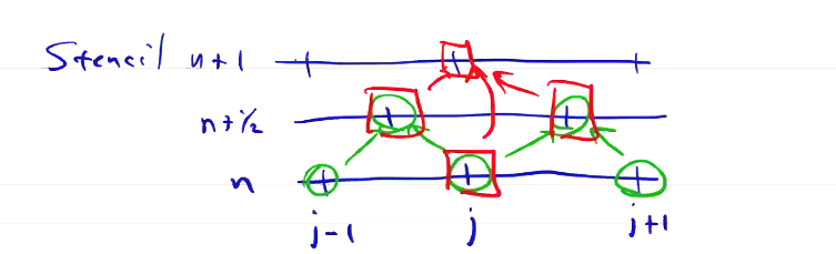
If we write out the stencil for Lax-Wendroff, we see that the algorithm is properly centered
For linear equations, the two steps can be combined, and we can see that it’s nothing but the combination of FTCS with a diffusion term
\[u_j ^{n+1} = u_j ^n - \underbrace{\frac{a \Delta t}{2 \Delta x} \left( u_{j + 1} ^n - u_{j - 1} \right)}_ {\text{FTCS}} + \underbrace{\frac{a^2 \Delta t^2}{2 \Delta x ^2} \left( u_{j+1} ^n - 2 u_j ^n + u_{j - 1} ^n \right)} _{\text{Diffusion}}\]which approximates the PDE
\[\pdv{u}{t} + a \pdv{u}{x} = \frac{a^2 \Delta t}{2} \pdv{^2 u}{x ^2}\]Lax-Wendroff has an accuracy of \( \mathcal{O}(\Delta t ^2, \Delta x^2) \). Because of this, it’s a very useful algorithm.
If the system is non-linear, then we do apply Lax-Wendroff as a 2-step process. For instance, if we look at the form of the MHD equations,
\[\pdv{\vec Q}{t} + \pdv{\vec F}{x} = 0\]The first Lax advance will be
\[Q_{j + 1/2} ^{n + 1/2} = \frac{Q_{j + 1} ^n + Q_j ^n}{2} - \frac{\Delta t}{2 \Delta x} \left( F_{j + 1} ^n - F_j ^n \right)\]and the leapfrog advance is
\[Q_j ^{n + 1} = Q_j ^n - \frac{\Delta t}{\Delta x} \left( F_{j + 1/2} ^{n + 1/2} - F_{j - 1/2} ^{n + 1/2} \right)\]There is a way to generalize the Lax-Wendroff procedure, which produces the class of Lax-Wendroff-type algorithms. To step from \( n \) to \( n + 1 \), we first compute the solution at an intermediate step \( n + \alpha \) at some intermediate grid points \( j + \beta \). These algorithms are described by the stencil:
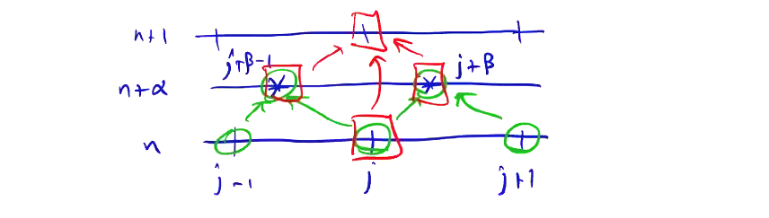
For \( \alpha = \beta = \frac{1}{2} \), we get the Lax-Wendroff algorithm we just described. There’s another useful algorithm known as the MacCormack algorithm, for which \( \alpha = 1, \beta = 0 \):
\[\overline{Q}_j = Q _j ^n - \frac{\Delta t}{\Delta x} \left( F_{j + 1} ^n - F_{j} ^n \right) \quad \text{(predictor step)}\] \[\overline{\overline{Q}}_j = Q_j ^n - \frac{\Delta t}{\Delta x} \left( \overline{F}_j - \overline{F} _{j - 1} \right) \quad \text{(corrector step)}\] \[Q_j ^{n + 1} = \frac{\overline{Q}_j + \overline{\overline{Q}}_j}{2} = \frac{\overline{Q}_j + Q_j ^n}{2} - \frac{\Delta t}{2 \Delta x} \left( \overline{F}_j - \overline{F}_{j - 1} \right)\] where \( \overline{F}_j = F(\overline{Q}_j) \). The MacCormack algorithm is also \( \mathcal{O}(\Delta t ^2, \Delta x ^2) \). In some cases it can be better (more stable) for multi-dimensional problems.
We’ve written these algorithms out in 1D. In 3D MHD, we can write out our system of equations as:
\[\pdv{\vec Q}{t} + \pdv{\vec F}{x} + \pdv{\vec G}{y} + \pdv{\vec H}{z} = 0\]We can write the predictor step as
\[\overline{Q} _{i,j,k} = Q^n _{i,j,k} - \frac{\Delta t}{\Delta x} \left( F _{i+1, j, k} - F _{i, j, k} ^n \right) - \frac{\Delta t}{\Delta y} \left( G _{i, j+1, k} - G _{i, j, k} ^n \right) - \frac{\Delta t}{\Delta z} \left( H _{i, j, k+1} - H _{i, j, k} ^n \right)\]and the corrector step as
\[\begin{aligned} \overline{\overline{Q}}_{i, j, k} & = & Q _{i, j, k} ^n - \frac{\Delta t}{\Delta x} \left( \overline{F}_{i, j, k} - \overline{F}_{i-1, j, k} \right) - \frac{\Delta t}{\Delta y} \left( \overline{F}_{i, j, k} - \overline{F}_{i, j-1, k} \right) \\ & & - \frac{\Delta t}{\Delta z} \left( \overline{F}_{i, j, k} - \overline{F}_{i, j, k-1} \right) \end{aligned}\] \[Q_{ijk} ^{n + 1} = \frac{\overline{Q} + \overline{\overline{Q}}}{2} \]To ensure stability, the domain of dependence must be contained in the numerical domain of dependence. If we plot out the slope of the zone of dependence, the physical domain has a slope \( |1 / \lambda_{max}| \), while the numerical domain has a slope \( |\Delta t / \Delta x| \):
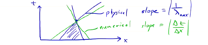
which gives us the stability condition: \[\frac{\Delta t}{\Delta x} \left| \lambda _{max} \right| \leq 1\]
where \( \lambda_{max} \) is the maximum eigenvalue of the flux Jacobian \( \pdv{\vec F}{\vec Q} \). In 2D, we have
\[\frac{\Delta t}{\Delta x} \left| \lambda _{A, max} \right| + \frac{\Delta t}{\Delta y} \left| \lambda _{B, max} \right| \leq 1\]where \( \vec A = \pdv{\vec F}{\vec Q} \) and \( \vec B = \pdv{\vec G}{\vec Q} \).
In standard gas dynamics, where the situation is much simpler, the eigenvalues are \( \lambda_A = (u, u + v_s, u - v_s) \), where \( v_s \) is the sound speed. The stability condition is then:
\[\Delta t \leq \left( \frac{|u| + v_s}{\Delta x} + \frac{|v| + v_s}{\Delta y} \right)\]For high speed flows, which have \( v > \lambda \) for any of the characteristic speeds, sometimes additional diffusion is necessary:
\[\pdv{\vec Q}{t} + \pdv{\vec F}{x} + \pdv{\vec G}{y} + \pdv{\vec H}{z} = \sigma \grad ^2 \vec Q\]This diffusivity can be added after we perform an update. For example, for the 2D MacCormack algorithm we can write
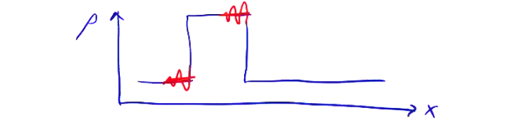
\[\left( Q_{i, j} ^{n + 1} \right)' = Q_{ij} ^{n + 1} + \Delta t \sigma \left[ \frac{\left( Q_{i + 1, j} ^{n + 1} - 2 Q_{i, j} ^{n + 1} + Q_{i-1, j} ^{n + 1}\right)}{\Delta x^2} + \frac{\left( Q_{i, j+1} ^{n + 1} - 2 Q_{i, j} ^{n + 1} + Q_{i, j-1} ^{n + 1}\right)}{\Delta y^2}\right]\]This helps to smooth out the oscillations that can result from a steep change in \( Q \):
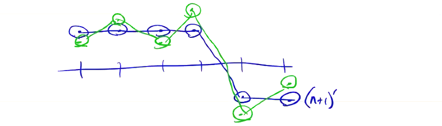
We can set \( \sigma \) to a constant everywhere, and a typical value might be
\[\frac{\sigma \Delta t}{\Delta x^2} < 0.25\]You can also make \( \sigma \propto \div \vec v \), so that we only add diffusion in the region of shocks or supersonic flows.
Method 2: Upwind Difference Flux#
Going back to our model equation can write the advection equation as
\[\pdv{u}{t} + a \pdv{u}{x} = 0\] \[\pdv{u}{t} + \pdv{f}{x} = 0 \qquad (f = au)\]
The simple upwind difference is expressed as
\[u_j ^{n+1} = u_j ^n - \frac{a \Delta t}{\Delta x} \begin{cases} (u_j ^n - u_{j-1} ^n) \quad &\text{if}& a \geq 0 \\ (u_{j+1} ^n - u_{j} ^n) \quad &\text{if}& a \geq 0 \end{cases}\]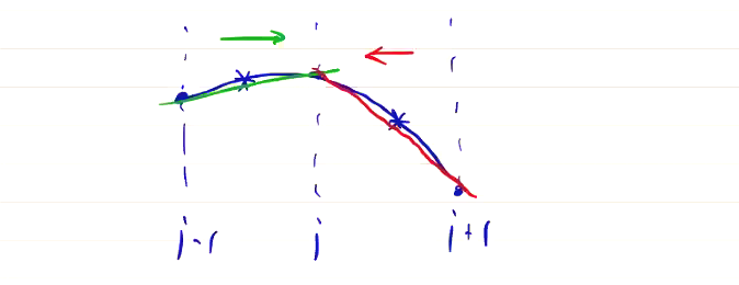
This works easily enough for the advection equation, but it does not work in general for systems of equations, because we can characteristics which are both positive and negative. We can not, for example, write
\[Q_j ^{n+1} = Q_j ^n - \frac{\Delta t}{\Delta x} \begin{cases} (F_j ^n - F_{j-1} ^n) \quad &\text{if} \quad \lambda \geq 0 \\ (F_{j+1} ^n - F_{j} ^n) \quad &\text{if} \quad \lambda < 0 \end{cases}\]Because in general \( \lambda_i \) will take both positive and negative values. In gas dynamics, \( \lambda = (v, v + v_s, v - v_s) \). In ideal MHD, we have seven waves:
\[\lambda = v, v \pm v_A, v \pm v_{\text{fast}}, v \pm v_{\text{slow}}\]From a point \( Q_j ^n \), waves of each of the characteristics propagate within their own domains:
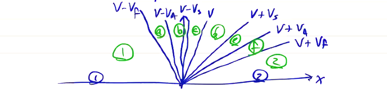
In regions \( (1) \) and \( (2) \), no information can propagate faster than the fastest characteristic \( (v \pm v_f) \). At any point in time, we can draw a horizontal line to see the extent of each domain. At any point in time, some eigenvalues are positive and some are negative. As drawn, \( v - v_f \) and \( v - v_A \) are negative, and the rest are positive.
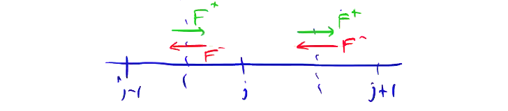
To apply an upwind difference, we must split the flux into right- and left-going components
\[F = F^+ + F^-\]Re-writing our original PDE:
\[\pdv{Q}{t} + \pdv{F}{x} = 0\] \[\pdv{Q}{t} + \pdv{F^+}{x} + \pdv{F^-}{x} = 0\]
we can now apply upwind differencing
\[\frac{Q_j ^{n+1} - Q_j ^n}{\Delta t} + \frac{F_j ^+ - F_{j - 1} ^+}{\Delta x} + \frac{F_{j+1} ^- - F_j ^- }{\Delta x} = 0\]To split \( F \) into \( F^+ \) and \( F^- \), we manipulate the original PDE using the flux Jacobian.
\[\pdv{Q}{t} + \pdv{F}{Q} \pdv{Q}{x} = 0\] \[\rightarrow \pdv{Q}{t} + A^+ \pdv{Q}{x} + A^- \pdv{Q}{x} = 0\]
where now \( A^+ \) and \( A^- \) are the flux Jacobians of \( F^+ \) and \( F^- \). The eigenvalue decomposition of \( A \) is
\[A X = X \Lambda\]where \( \Lambda \) is the diagonal matrix of eigenvalues and \( X \) is the matrix of eigenvectors. This means we can write \( A \) as
\[A = X \Lambda X^{-1}\]We can split our PDE into right- and left-going components as:
\[\pdv{Q}{t} + X \Lambda X^{-1} \pdv{Q}{x} = 0\] \[\pdv{Q}{t} + X \Lambda ^+ X^{-1} \pdv{Q}{x} + X \Lambda ^- X^{-1} \pdv{Q}{x} = 0\]
where \( \Lambda ^+ \) is the diagonal matrix of only right-going eigenvalues, and \( \Lambda^- \) is a diagonal matrix of only right-going eigenvalues.
For gas dynamics, the eigenvalues are \( v, v \pm v_s \) with \( 0 < v < v_s \)
\[\Lambda = \begin{bmatrix} v & 0 & 0 \\ 0 & v + v_s & 0 \\ 0 & 0 & v - v_s \end{bmatrix} \\ = \Lambda ^+ + \Lambda ^-\] \[\Lambda ^+ = \begin{bmatrix} v & 0 & 0 \\ 0 & v + v_s & 0 \\ 0 & 0 & 0 \end{bmatrix}\] \[\Lambda ^- = \begin{bmatrix} 0 & 0 & 0 \\ 0 & 0 & 0 \\ 0 & 0 & v - v_s \end{bmatrix}\]
Now we can properly upwind difference the flux by defining the flux at grid midpoints, computing \( F^+ \) based on \( F_j \), and computing \( F^- \) based on \( F_{j+1} \).
By defining the numerical flux at the grid midpoints, this naturally leads to a finite volume implementation.
Finite Volume Method#
Finite volume methods differ from finite difference methods in the quantity which we store at each grid point. If we consider a volume centered at grid point \( j + 1/2 \), we can integrate over the cell volume to get the average value of the function over the volume.
\[\pdv{}{t} \underbrace{\int _\Omega \vec Q \dd \vec V} _ {\int _\Omega \rho \dd \vec V = m _\Omega} + \underbrace{\int _ \Omega \div \vec F \dd \vec V = 0} _{\oint \dd \vec S \cdot \vec F \rightarrow \sum_{\text{sides}} \vec S _j \cdot \vec F _j }\]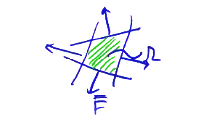
Because the integral is determined by the fluxes, which are defined along the cell edges rather than the grid points, this sort of method is no longer constrained to evenly-spaced quadrilateral grids. Much more complicated polygons are possible, allowing us to avoid the stair-stepping issues at the boundary of uniform grids.
Fluxes are computed using the upwind method
\[F_{j + 1/2} = F^- _{j + 1} + F_j ^+ = \vec X \vec \Lambda ^- \vec X ^{-1} Q_{j+1} + \vec X \vec \Lambda^+ \vec X^{-1} Q_j\]Manipulating this a bit, we can get a more convenient form for evaluating the fluxes. \[F_{j + 1/2} = \vec X \underbrace{\left( \frac{ \vec \Lambda - |\vec \Lambda|}{2} \right)}_{\text{negative components}} \vec X^{-1} Q_{j+1} + \vec X \underbrace{\left( \frac{\vec \Lambda + |\vec \Lambda| }{2} \right)}_{\text{positive components}} \vec X^{-1} Q_j \\ = \frac{1}{2} \left( \vec X \vec \Lambda \vec X^{-1} Q_{j+1} + \vec X \vec \Lambda \vec X^{-1} Q_j \right) - \frac{1}{2} \vec X | \vec \Lambda| \vec X^{-1} (Q_{j+1} - Q_j) \\ = \underbrace{\frac{F_j + F_{j+1}}{2}}_{\text{Centered flux}} - \underbrace{\frac{1}{2} \left( \vec X |\vec \Lambda| \vec X ^{-1} \right) _{j + 1/2} (Q_{j+1} - Q_j)}_{\text{Flux correction}}\]
To calculate \( \vec X |\vec \Lambda | \vec X^{-1} \) at grid point \( j + 1/2 \), we need to perform some sort of average between \( Q_j \) and \( Q_{j+1} \). The simplest is just:
\[Q_{j+1/2} = \frac{Q_j + Q_{j+1}}{2}\]which isn’t conservative, but works pretty well. There are other averaging methods, like the Roe average, that attempt to preserve conservative properties by propagating a density average through \( Q \).
This is called an Approximate Riemann Solver. It’s composed of two separate steps, a centered flux (unstable FTCS), and a flux correction based on the characteristics of the PDE (stable).
Equilibrium Calculations#
From physical expectations, elliptic equations result from equilibrium calculations and eigenvalue systems. In general, we can write elliptic equations as \[\vec A \vec x = \vec b\] where \( \vec A \) may be a nonlinear function of \( \vec x \). For example, if we think of Poisson’s equation in 1D, \[\dv{^2 \phi}{x^2} = - \rho_c\] and apply finite differencing, \[\frac{\phi_{j+1} - 2 \phi_j + \phi_{j-1}}{\Delta x^2} = - \rho_j\] we get a matrix system \[\vec A \vec x = \frac{1}{\Delta x^2} \begin{bmatrix} -2 & 1 & 0 & \ldots \\ 1 & -2 & 1 & \ldots \\ \ldots & \ldots & \ldots & \ldots \end{bmatrix} \begin{bmatrix} \phi_1 \\ \phi_2 \\ \ldots \end{bmatrix} = \vec b = - \begin{bmatrix} \rho_1 \\ \rho_2 \\ \ldots \end{bmatrix}\] where \( \vec A \) is a J by J matrix. In equilibrium calculations, this comes up when solving the Grad-Shafranov equation
\[\Delta ^\star \psi = I I' - \mu_0 r^2 p'\] where \[I' = \pdv{I}{\psi} \qquad p' = \pdv{p}{\psi}\] and \[\Delta ^\star \equiv r \pdv{}{r} \frac{r}{r} \pdv{}{r} + \pdv{^2}{z^2}\]
The Grad-Shafranov equation is a nonlinear equation, and we often assume a power series expansion of the current density and pressure \[I(\psi) = I_0 + I_1 \psi + I_2 \psi^2 + \ldots\] \[p(\psi) = p_0 + p_1 \psi + p_2 \psi^2 + \ldots\]
For a force-free equilibrium (\( p = 0 \)) with a linear current profile \[I I' = I_0 I_1 + I_1 ^2 \psi\]
this makes the Grad-Shafranov equation a linear system. \[\vec A = \Delta ^\star _{\text{FD}} + I_1 ^2\] \[\vec x = \psi_{ij} \qquad \vec b = (I_0 I_1) _{ij}\] where \( \Delta ^\star _{\text{FD}} \) is a finite difference representation of the \( \Delta ^\star \) operator. For a given geometry and poloidal current profile, \( I_0 \) and \( I_1 \), we can solve \( \vec A \vec x = \vec b \) to give \( \psi(r, z) \).
Solving \( \vec A \vec x = \vec b \) can be done using either direct or indirect (iterative) methods. Direct decomposition methods (like Kramer’s rule, Gaussian decomposition) require \( \mathcal{O}(N^3) \) operations, where \( N \) is the size of the matrix. They also require full matrix storage, even though \( \vec A \) is a sparse (tridiagonal) matrix.
Iterative methods help solve this problem. We begin with a solution which is improved upon until we get convergence. If this converges in fewer operations than a full decomposition, then we’ve saved some time and a lot of in-memory storage space.
\[x^0 \rightarrow x^1 \rightarrow x^2 \rightarrow \ldots\] \[\vec x^{n+1} = \vec x^n + \vec B^{-1} (\vec b - \vec A \vec x^n) \\ = \vec x^n + \vec B^{-1} \vec r^n\]
The technique boils down to a clever choice of \( \vec B \). We want to choose an approximation matrix \( \vec B \) which is very close to \( \vec A \), but is much easier to invert. \[\vec B \approx \vec A\] For this kind of iterative method, each iteration requires \( \mathcal{O}(N) \) operations, and converges in fewer than \( N \) iterations. The best iterative methods can converge in \( \mathcal{O}(N \ln N) \) total operations.
Linear Stability#
When we studied plasma waves at the beginning of this course, we performed a linearization of the Vlasov equation about an equilibrium state. This is how we got dispersion relations for waves. We assumed an equilibrium of a uniform plasma, with at most static magnetic fields. For more interesting equilibria with nonzero gradients, we follow the same procedure.
First, we linearize the ideal MHD equations about a static equilibrium (\( \vec v_0 = 0 \)) \[\pdv{\rho_1}{t} = - \div (\rho_0 \vec v_1)\] \[\pdv{p_1}{t} = - \div (p_0 \vec v_1) + (1 - \Gamma) p_0 \div \vec v_1\] \[\pdv{\vec B_1}{t} = \curl (\vec v_1 \cross \vec B_0)\] \[\rho _0 \pdv{\vec v_1}{t} + \frac{1}{\mu_0} \left[(\curl \vec B_1) \cross \vec B_0 + (\curl \vec B_0) \cross \vec B_1 \right]\]