MHD Equilibrium Calculations #

From physical expectations, elliptic equations result from equilibrium calculations and eigenvalue systems. In general, we can write elliptic equations as \[\vec A \vec x = \vec b\] where \( \vec A \) may be a nonlinear function of \( \vec x \). For example, if we think of Poisson’s equation in 1D, \[\dv{^2 \phi}{x^2} = - \rho_c\] and apply finite differencing, \[\frac{\phi_{j+1} - 2 \phi_j + \phi_{j-1}}{\Delta x^2} = - \rho_j\] we get a matrix system \[\vec A \vec x = \frac{1}{\Delta x^2} \begin{bmatrix} -2 & 1 & 0 & \ldots \\ 1 & -2 & 1 & \ldots \\ \ldots & \ldots & \ldots & \ldots \end{bmatrix} \begin{bmatrix} \phi_1 \\ \phi_2 \\ \ldots \end{bmatrix} = \vec b = - \begin{bmatrix} \rho_1 \\ \rho_2 \\ \ldots \end{bmatrix}\] where \( \vec A \) is a J by J matrix. In equilibrium calculations, this comes up when solving the Grad-Shafranov equation

\[\Delta ^\star \psi = I I' - \mu_0 r^2 p'\] where \[I' = \pdv{I}{\psi} \qquad p' = \pdv{p}{\psi}\] and \[\Delta ^\star \equiv r \pdv{}{r} \frac{r}{r} \pdv{}{r} + \pdv{^2}{z^2}\]

The Grad-Shafranov equation is a nonlinear equation, and we often assume a power series expansion of the current density and pressure \[I(\psi) = I_0 + I_1 \psi + I_2 \psi^2 + \ldots\] \[p(\psi) = p_0 + p_1 \psi + p_2 \psi^2 + \ldots\]

For a force-free equilibrium (\( p = 0 \)) with a linear current profile \[I I' = I_0 I_1 + I_1 ^2 \psi\]

this makes the Grad-Shafranov equation a linear system. \[\vec A = \Delta ^\star _{\text{FD}} + I_1 ^2\] \[\vec x = \psi_{ij} \qquad \vec b = (I_0 I_1) _{ij}\] where \( \Delta ^\star _{\text{FD}} \) is a finite difference representation of the \( \Delta ^\star \) operator. For a given geometry and poloidal current profile, \( I_0 \) and \( I_1 \), we can solve \( \vec A \vec x = \vec b \) to give \( \psi(r, z) \).

Solving \( \vec A \vec x = \vec b \) can be done using either direct or indirect (iterative) methods. Direct decomposition methods (like Kramer’s rule, Gaussian decomposition) require \( \mathcal{O}(N^3) \) operations, where \( N \) is the size of the matrix. They also require full matrix storage, even though \( \vec A \) is a sparse (tridiagonal) matrix.

Iterative methods help solve this problem. We begin with a solution which is improved upon until we get convergence. If this converges in fewer operations than a full decomposition, then we’ve saved some time and a lot of in-memory storage space.

\[x^0 \rightarrow x^1 \rightarrow x^2 \rightarrow \ldots\] \[\vec x^{n+1} = \vec x^n + \vec B^{-1} (\vec b - \vec A \vec x^n) \\ = \vec x^n + \vec B^{-1} \vec r^n\]

The technique boils down to a clever choice of \( \vec B \). We want to choose an approximation matrix \( \vec B \) which is very close to \( \vec A \), but is much easier to invert. \[\vec B \approx \vec A\] For this kind of iterative method, each iteration requires \( \mathcal{O}(N) \) operations, and converges in fewer than \( N \) iterations. The best iterative methods can converge in \( \mathcal{O}(N \ln N) \) total operations.

Linear Stability #

When we studied plasma waves at the beginning of this course, we performed a linearization of the Vlasov equation about an equilibrium state. This is how we got dispersion relations for waves. We assumed an equilibrium of a uniform plasma, with at most static magnetic fields. For more interesting equilibria with nonzero gradients, we follow the same procedure.

First, we linearize the ideal MHD equations about a static equilibrium (\( \vec v_0 = 0 \)) \[\pdv{\rho_1}{t} = - \div (\rho_0 \vec v_1)\] \[\pdv{p_1}{t} = - \div (p_0 \vec v_1) + (1 - \Gamma) p_0 \div \vec v_1\] \[\pdv{\vec B_1}{t} = \curl (\vec v_1 \cross \vec B_0)\] \[\rho _0 \pdv{\vec v_1}{t} = \grad p_1 + \frac{1}{\mu_0} \left[(\curl \vec B_1) \cross \vec B_0 + (\curl \vec B_0) \cross \vec B_1 \right]\]

Given an equilibrium (\( \rho_0 \), \( p_0 \), \( \vec B_0 \)), the linearized MHD equations can be integrated in time to evolve \( \rho_1 \), \( p_1 \), \( \vec B_1 \), \( \vec v_1 \). If we do this and \( \vec v_1 \) grows in time, then the plasma is unstable.

Notice that \( \rho_1 \) decouples from the other equations, so we don’t need to evolve it if we don’t want to, or we can evolve it in parallel.

It’s often more useful to study individual modes. We can assume a form of the perturbation to select specific modes. For arbitrary perturbed quantity \( g_1 \),

where \( m \) is the azimuthal mode number. As we’ve written it, \( g_1 \) is complex-valued, but only because \( e^{i m \theta} \) is a convenient representation of a Fourier mode. We’re only interested in the real component.

\[\text{Re}(g_1) \leftrightarrow g_1(\theta = 0)\] \[\text{Im}(g_1) \leftrightarrow g_1(\theta = - m \pi / 2)\]

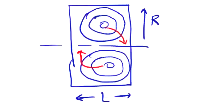
Example: Spheromak Tilt m=1 #

As an example, we consider the \( m=1 \) tilt mode in the spheromak, a device which consists of a toroidal equilibrium contained in a cylindrical can. The tilt mode, corresponding to \( m=1 \), rotates the equilibrium in the \( r-z \) plane. The elongation ratio \( L/R \) determines the configuration’s stability against the tilt mode.

(stable: L/R=1, unstable: L/R=2)

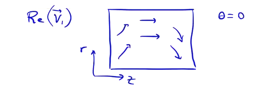
Plotting the real part of \( g \) in the \( r-z \) plane at \( \theta = 0 \) looks something like this:

We can fill out the lower half of the plane at “\( r < 0 \)” by setting \( \theta = \pi \), so we get the negative of the upper half

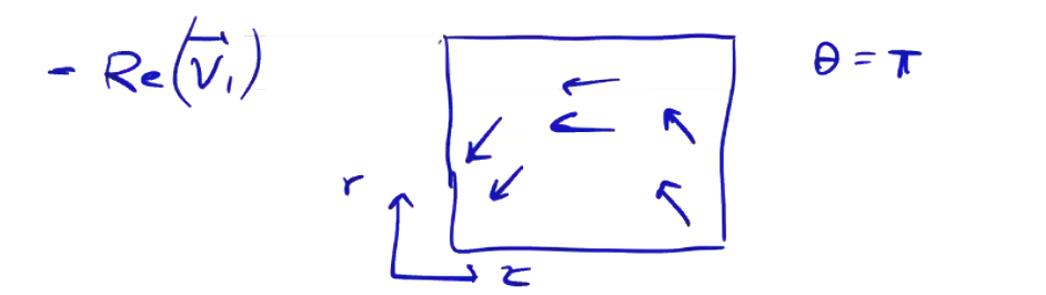
To align the \( r \) axes, we need to flip this upside-down before we can put it on the same axes as the upper \( r-z \) plane.

The assumed form is implemented in the linear equations. Noting:

The remaining terms are approximated with finite differences.

We can construct the other difference relations for the other perturbed quantities from the linearized ideal MHD equations:

\[{p_1}_{ij} ^{n+1} = {p_1}_{ij} ^n + \Delta t \left[ \ldots \right]^n\] \[{\vec B_1}_{ij} ^{n+1} = {\vec{B_1}}_{ij} ^n + \Delta t [ \ldots ] ^n\] \[{\vec v_1} _{ij} ^{n+1} = {\vec v_1}_{ij} ^{n+1} + \Delta t [\ldots ]^n\]

Normalization #

We normalize the PDE’s by nondimensionalizing. We do this by choosing characteristic values for density, pressure, magnetic field, velocity

\[\rho_0 = \tilde{\rho_0} \rho ^\star \qquad \text{where} \quad \tilde{\rho_0} \in [0, 1] \] \[\rho_1 = \tilde{\rho_1} \rho^\star\] \[p_0 = \tilde{p_0} p^\star\] \[\vec B_0 = \tilde{\vec B} B^\star\] \[\vec v_1 = \tilde{\vec v_1} v^\star \qquad v^\star = L / \tau\]

We can combine into a single PDE by taking the time derivative of the momentum equation, such that the sound speed and Alfven speed fall out:

\[\pdv{ ^2 \tilde{\vec v_1}}{\tilde t ^2} = \frac{\tau ^2}{L^2} \frac{\Gamma p^\star}{\rho ^\star} f_a (\tilde{\rho}_0, \tilde{p}_0, L/R, \tilde{\vec{v}}_1) + \frac{\tau^2}{L^2} \frac{{B^\star} ^2}{\mu_0 \rho^\star} f_b(\tilde{\rho}_0, \tilde{\vec B}_0, L/R, \tilde{\vec v}_1)\] \[\frac{\Gamma p^\star}{\rho ^\star} = v_s ^2 \qquad \frac{{B^\star}^2}{\mu_0 \rho ^\star}\]

here \( f_a \) and \( f_b \) are some appropriate conversion functions.

In our nondimensionalization, we normalize \( z \) and \( r \) by characteristic lengths \( L \) and \( R \):

\[t = \tilde t \tau\] \[z = \tilde z L\] \[r = \tilde r R = \frac{\tilde r L}{L/R}\]

Initial Conditions #

To solve for the evolution of a perturbation in time, we need initial conditions. The initial condition is both the equilibrium \( \rho_0, p_0, \vec B_0, \vec v_0 = 0 \) and the perturbation \( \vec v_1 (r, z) \). For stability analysis, we generally want our perturbation to excite all modes (or as many as possible), and avoid single mode perturbations. The dominant mode will grow the fastest, and we’ll see it come out of the excitation.

You don’t want to perturb a magnetic field that breaks \( \div \vec B_1 = 0 \). In generall, you can just perturb the velocity \( \vec v_1 (r, z) \), for example like this \[\text{Re}(\vec v_1) \propto \sin \left( \frac{\pi r}{R} \right) \cos \left( \frac{\pi z}{L} \right)\] Because we generally don’t expect a radial dependence to be a sin function, \( \sin (\pi r / R) \) should excite many modes. We also need to meet the boundary conditions, hence using functions with easy to compute zeroes.

We the advance the solution in time, and track the evolution of the perturbed kinetic energy

If the equilibrium is unstable, then a dominant mode will grow out of the oscillations with a measurable growth rate \( \gamma \)

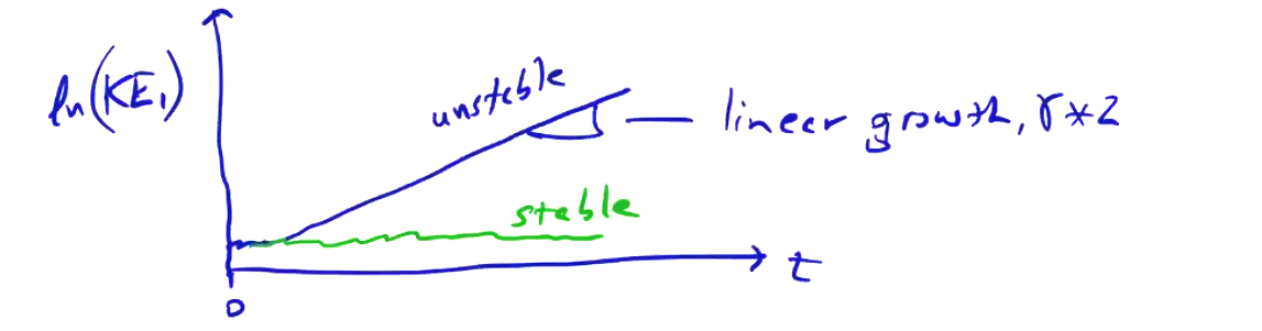
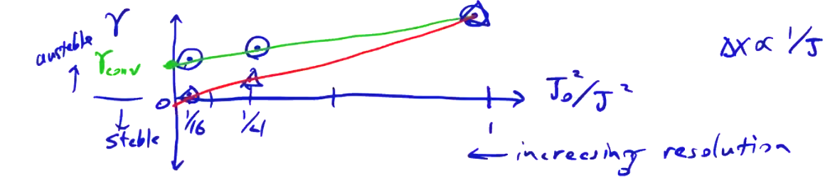
To study the accuracy order and compare with results, we need to perform a convergence study of the growth rate. We do this by performing the simulation with different grid resolutions. If we plot against some kind of normalized grid resolution \( J_0 ^2 / J ^2 \), where \( J \) is the most coarse grid resolution. We expect second-order convergence, so plotting the square of the resolution should give us straight lines moving towards zero.

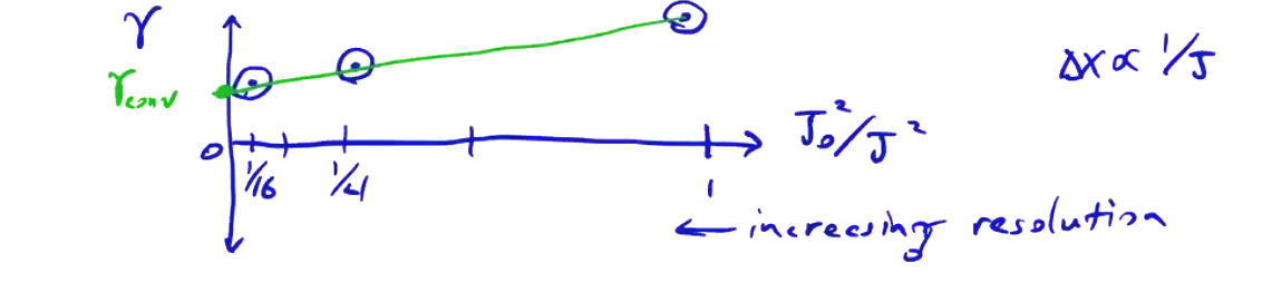
The difference between points as we move to higher resolution gives a bound on the error. We may also find solutions that appear to be unstable, but the projected growth rate is zero (or close to it)

The eigenfunction \( \vec v_1 \) itself contains useful information, since it describes the unstable behavior. In the m=1 spheromak case, it indicates that the spheromak will tilt. There are other modes that shift the configuration. The difference between these can be seen by looking at the eigenfunction itself.

The advantages of this time integration method are:

• Simple to implement.
• The approach is general to many equilibria.

Some of the disadvantages are

• Requires a choice of \( \Delta t \) (eigenvalue problem)
• Marginal stability boundaries are difficult to determine exactly.

Boundary Conditions for Stability Analysis #

For a rigid conducting wall,

\[\pdv{}{t} \vec B_1 \cdot \vu n = 0 \qquad \text{or, usually} \quad \vec B_1 \cdot \vu n = 0\] \[\vec v_1 \cdot \vu n = 0\]

Scalar quantities (\( \rho_1 \), \( p_1 \)) are set to zero at the boundaries.

There are also axis conditions in cylindrical geometry, where \( r = 0 \). For axis boundaries, we want to assume that all variables are analytic at the axis. That is, there are no singularities, and the solution is differentiable. Then, we want to map from the \( r \)-\( \theta \) plane to an \( x \)-\( y \) plane. The \( z \) direction is a trivial one-to-one mapping. Then, we expand in a power series such that:

Ordinarily, you would extend this out to more terms than this, but in this case we happen to already know how many terms we need. Then, map to the cylindrical coordinates:

\[A_r = A_x \cos \theta + A_y \sin \theta \qquad x = r \cos \theta\] \[A_\theta = - A_x \sin \theta + A_y \cos \theta \qquad y = r \sin \theta\]

Substituting in the expanded quantities gives:

The solution behavior at the axis \( r \rightarrow 0 \) depends on the \( \theta \) resolution. We assumed \( A \propto e^{i m \theta} \), or

where \( \vec A ^r \) is the real component of \( \vec A \). If we consider axisymmetric modes, \( m = 0 \), based on this expression we have no \( \theta \) dependence \[\vec A = \vec A^r\]

We set the appropriate coefficients to match the expansion. If there is no \( \theta \) dependence, each part of our expansion for \( A_r \), \( A_\theta \), \( A_z \) which has a \( \theta \) dependence must vanish:

\[A = D = B - F = C + E = H = J = K = L = 0\] so \[B = F \qquad \text{and} \qquad C = - E\]

which gives

\[A_r = Br \] \[A_\theta = Er\] \[A_z = G \]

as \( r \rightarrow 0 \). So the boundary conditions at the axis are:

\[\left.A_r \right|_{\text{axis}} = 0\] \[\left.A_\theta \right|_{\text{axis}} = 0\]

For \( m = 1 \), \( \vec A = \vec A ^r \cos \theta - \vec A^i \sin \theta \)

gives

\[B + F = B - F = C + E = E - C = G = K = L = 0\] \[B = F = C = E = 0\] which gives \[A_r = A \cos \theta + D \sin \theta\] \[A_\theta = D \cos \theta - A \sin \theta\] \[A_z = H r \cos \theta + J r \sin \theta\]

So the boundary conditions are

\[\left. \pdv{A_r}{r} \right|_{\text{axis}} = 0\] \[\left. \pdv{A_\theta}{r} \right|_{\text{axis}} = 0\] \[\left. A_z \right|_{\text{axis}} = 0\]

Note, the real component of the \( r \) component is the \( \theta \) component of the imaginary component \[A_r ^r = A_\theta ^i\] and \[A_\theta ^r = - A_r ^i\]

We can do the same thing for other mode numbers, and arrive at a general correspondence. Scalar variables map in the same way the axial component \( A_z \).

Questions??

Setting up the initial conditions:

• what goes in “e”?
• calculate B_x, B_y from J_z?