Mathematical review#
We’re starting off with some mathematical foundation to ensure we’re all on the same page before we start talking about waves and collisions.
Fourier Series / Spectral Analysis#
First, let’s not get confused between Fourier series and Fourier transforms. A Fourier series is the breakdown of a function defined on a finite interval into “frequency components.” For example, if we have \( f(x) : x \in [a, b] \), a Fourier series for \( f(x) \) pulls apart the discrete frequency components of the \( e^{ikx} \) modes that make up the function. Starting with a fundamental mode \( f_0 \), a first harmonic \( f_1 \), a second harmonic \( f_2 \), and so on and so forth. We won’t end up with any energy in the frequencies between those modes, since it’s a discrete series.
A Fourier transform is a transformation on a function on an infinite interval. When transformed, we end up with a continuous spectrum in frequency space. Same basic principles, but the important difference is a Fourier series is from a finite interval to a discrete spectrum.
There are also special geometries that don’t follow the basic 1D Fourier transformation. For example, if a function is defined on a disk (polar coordinates), then the eigenfunctions of the transform are the Bessel functions, and we perform spectral analysis via a “Bessel transform.” In a spherical geometry we have spherical Bessel functions.
Fourier’s important contribution was this: any arbitrarily capricious graph can be represented in the limit as a sum of sines and cosines. Fourier series are applicable in every area of physics. Why? Why are these trigonometric functions so applicable?
The complex exponentials \( e^{ikx} = \cos(kx) + i \sin(kx) \) are the eigenfunctions of 1D intervals. Every time we draw a graph on a continuous interval, these eigenfunctions are the “best” available basis for representing that graph on that interval. This makes more sense if we try to summarize Sturm-Liouville theory.
Sturm-Liouville Theory#
Sturm-Liouville is a mature, complete theory of evolutionary equations. We’ve talked about various types of evolution equations in basically every other section in these notes.
For example,
- Heat equation (diffusion): \( \pdv{u}{t} = D \pdv{^2u}{x} \)
- Advection: \( \pdv{u}{t} + a \pdv{u}{x} = 0 \)
- Advection-Diffusion (both): \( \pdv{u}{t} = \pdv{}{x}(D \pdv{u}{x}) + a \pdv{u}{x} \)
Any generic evolution equation relates the time derivative to a differential operator
\[\pdv{u}{t} = A u\]Sturm-Liouville is for all linear, 2nd-order operators \( A \). To make the notation a bit easier, let’s use \( u_t \equiv \pdv{u}{t} \), \( u_{xx} \equiv \pdv{^2u}{x^2} \)
The standard form of a 2nd-order linear equation is
\[\begin{aligned} u_t + f(t) u & = & a(x) u_{xx} + b(x) u_x + c(x) u \\ & = & A u \end{aligned}\]To solve the equation, we use separation of variables, where we say our solution will be a product of a function \( X(x) \) with all the spatial information and a function \( T(t) \) with all of the temporal information. When we substitute the solution, we find
\[(T' + f(x) T )X = T A X \\ \rightarrow \frac{AX}{X} = \frac{T' + f(t) T}{T}\]Because the left-hand-side depends only on \( x \) and the right-hand-side depends only on \( t \), they must be equal to some constant \( \lambda \). We get two equations, the first being the eigenvalue problem
\[AX = \lambda X\]and a temporal eigenvalue problem
\[T' = (\lambda - f(t) ) T\]We start with the the spatial one, because in general we will know the spatial boundary conditions for our problem (otherwise it’ll be rather difficult to solve!). For the 2nd order eigenvalue problem given sufficient boundary conditions for \( u \)
\[a(x) X'' + b(x) X' + (c(x) - \lambda) X = 0\]we can get to the standard form with an integrating factor
\[I(x) = \frac{1}{a(x)} \exp \left( \int ^x \frac{b(y)}{a(y)} \\dy \right)\] \[\dv{}{x} \left( a(x) I \dv{X}{x} \right) + I(x) \left( c(x) - \lambda \right)X = 0\]
This is the standard Sturm-Liouville form. Or, on the internet we’ll see the “standard Sturm-Liouville form” written slightly differently
\[\dv{}{x} \left( p(x) \dv{u}{x} \right) + q(x) u + \lambda w(x) u = 0\]This form is important because of a miraculous theorem:
\[\] Theorem Given regular boundary conditions on \( u(x) \) for \( x \in [a, b] \), the Sturm-Liouville equation has
- Distinct eigenvalues \( \lambda_n, n = 1, 2, \ldots \)
- For each eigenvalue \( \lambda_n \) there is an eigenfunction \( X_n \).
- The eigenfunctions form a complete set of orthogonal functions: \( \int _a ^b X_n X_m w(x) \dd x = 0, n \neq m \) (the weighting function \( w(x) \) is the above function in the standard S-L form). Completeness is the statement that one can expand any function on \( [a, b] \) using the set of eigenfunctions.
- With the temporal eigenfunctions \( T_n(t) \), the solution to the S-L equation is the sum of all the eigenfunctions \[u(x, t) = \sum_{n=1} ^{\infty} a_n X_n(x) T_n (t)\]
We start out with some temporal initial conditions
\[u_0 \equiv u(x, 0) = \sum_{n=1}^{\infty} a_n X_n(x)\]We get the weighting coefficients \( a_n \) by taking the inner product of each eigenfunction with the initial conditions:
\[\langle X_m | u_0 \rangle = \sum_{n=1} ^{\infty} a_n \langle X_m | X_n \rangle \\ = a_m \langle X_m | X_m \rangle \\ \rightarrow a_m = \frac{\langle X_m | u_0 \rangle}{\langle X_m | X_m \rangle}\]The completeness property of S-L gives families of orthogonal functions for any particular differential equation. The family we get ends up being a natural basis for physical situations.
Consider the Sturm-Liouville system:
- \( u^{\prime \prime} - \lambda ^2 u = 0 \) over the domain \( u \in [ -L / 2, L / 2] \)
We’ve got \( w(x) = 1 \) and inner product \( \langle X_n | X_m \rangle = \int _{-L/2} ^{L/2} X_n X_m \dd x \)
The eigenfunctions are \( \left[ \frac{1}{2}, \sin (\lambda _n x), \cos (\lambda_n x) \right] \) and the eigenvalues are \( \lambda_n = \frac{2 \pi}{L} n \)
The orthogonality relation says \[\langle u_n u_m \rangle = \int _{-L/2} ^{L/2} u_m (x) u_n (x) \dd x = 2 L \delta _{n m}\]
The Fourier basis is the simplest Sturm-Liouville system. It applies to systems that are on an interval and internally homogeneous.
There are other systems, like the Chebyshev, Hermite, and Laguerre polynomials. The only requirement is that the system satisfies a 2nd-order linear differential equation. But the Fourier basis satisfies the simplest possible 2nd-order S-L equation.
Back to Fourier series, let’s get the Fourier theorem:
Theorem: Any periodic function can be decomposed into a potentially infinite series of sine and cosine functions. If period is \( L \), that is (\( f(x + L) = f(x) \)), then
\[f(x) = \frac{a_0}{2} + \sum _{n=1} ^{\infty} a_n \cos (k_n x) + b_n \sin (k_n x)\]with frequencies/wavenumbers given by
\[k_n = \frac{2 \pi}{L} n, n = 1, 2, 3, \ldots\]and Fourier coefficients / expansion coefficients given by
\[a_n = \frac{2}{L} \int_0 ^L f(x) \cos (k_n x) \dd x\] \[b_n = \frac{2}{L} \int_0 ^L f(x) \sin (k_n x) \dd x\]
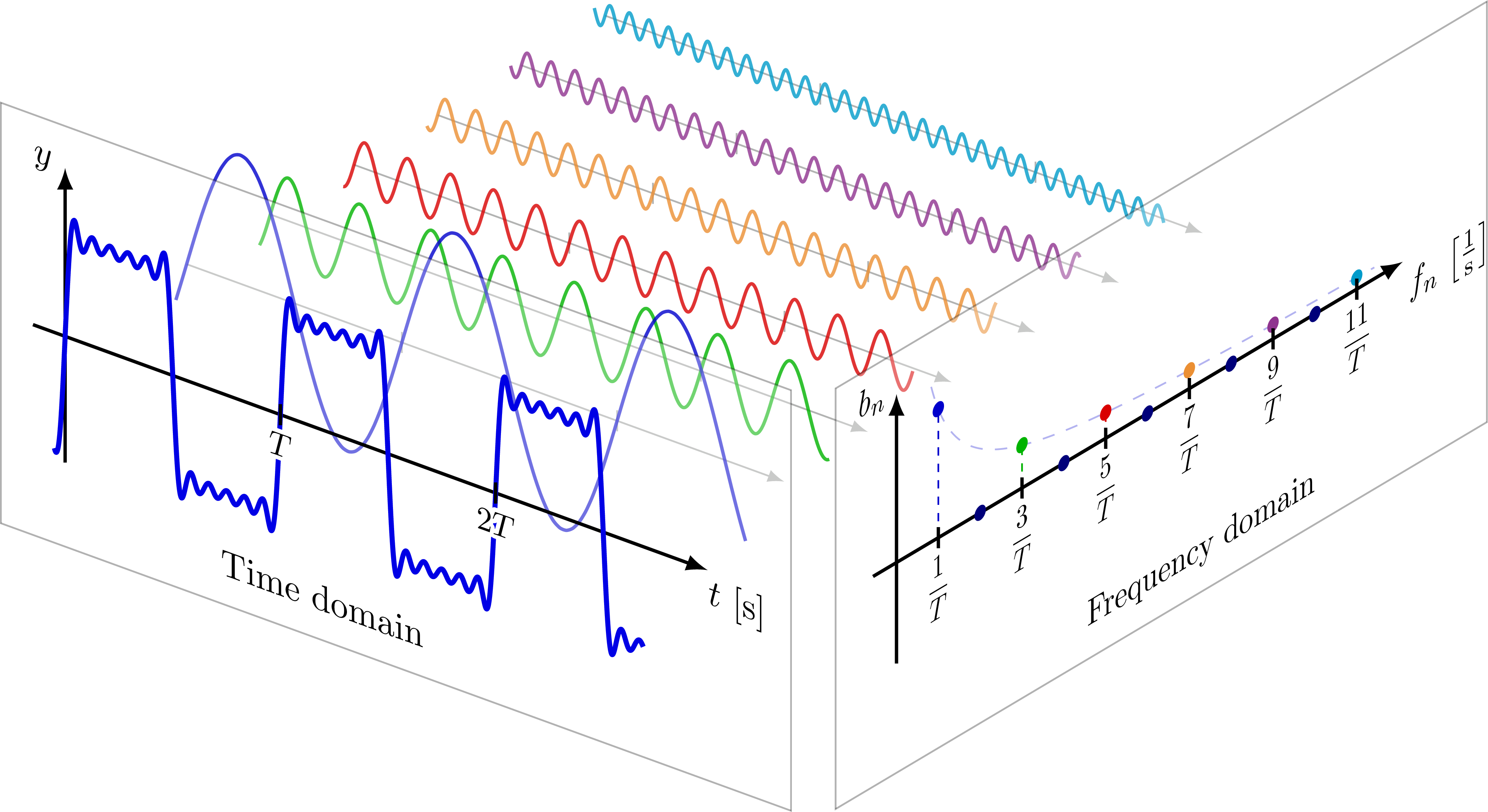
The set of coefficients \( a_n, b_n \) forms the spectrum of \( f(x) \). For the Fourier series to be convergent, the spectrum must decay sufficiently quickly, so we’ll see the coefficients getting smaller as \( n \rightarrow \infty \).
We usually express the Fourier series using the more convenient complex form by making use of the Euler identity \( e^{i k x} = \cos (kx) + i \sin (kx) \)
\[f(x) = \sum_{n = -\infty} ^{\infty} c_n e^{i k_n x}\] In this form we only have a single set of coefficients given by the Fourier integral \[c_n = \frac{1}{L} \int_0 ^L f(x) e ^{-i k_n x} \dd x\]
You can show that they are related to the previous ones by
\[ c_n = \frac{1}{2} (a_n - i b_n) \qquad n > 0 \\ = \frac{1}{2} (a_n + i b_n) \qquad n < 0>\]Let’s build some intuition by looking into some examples of Fourier spectra.
Series with finite spectra#
Simple Waveform
\[u = \sin (5x)\]By inspection,
\[\sin (5x) = \frac{1}{2i} \left( e^{i 5x} - e ^{-i 5 x} \right)\]That was easy, that’s the whole series. There are only two Fourier coefficients
\[c_5 = - \frac{i}{2} \qquad c_{-5} = \frac{i}{2}\]
Beat wave
\[u = \cos (6x) \cos (x)\]Expanding each of the cosines as complex exponentials
\[u = \frac{1}{4} \left( e^{i 6 x} + e^{- i 6 x} \right) (e^{ix} + e^{-ix})\] \[= \frac{1}{4} \left( e^{i 7 x} + e^{-i 7 x} + e^{i 5 x} + e^{-i 5 x} \right)\] \[= \frac{1}{2} \left( \cos (7x) + \cos (5x) \right)\]
So we’ve got four coefficients
\[c_{\pm 5} = \frac{1}{4}, \qquad c_{\pm 7} = \frac{1}{4}\]
Fourier series with infinite spectra#
Square Wave
\[f(x) = \begin{cases} 1 & \qquad & 0 < x < T/2 \\ -1 & \qquad & -T/2 < x < 0 \end{cases}\]This is about as discontinuous as you get. If you do the Fourier integrals, you get
\[f(x) = \sum_{n = \text{odd}} \frac{-i}{\pi n} e^{i k_n x}\] \[|c_n| \sim \frac{1}{n}\] The series has a slow convergence, and if you plot the spectrum you get a power law relationship.
Triangle Wave
The points of the triangle wave where the function is continuous but not differentiable give us a similarly slow convergence of the Fourier spectrum. For a triangle wave it ends up that
\[| c_n| \sim \frac{1}{n^2}\]so they converge an order faster than a square wave, but still very slowly.
Elliptic Cosine
Sort of like a cosine, except that it’s defined on an ellipse instead of a circle. We give it some parameter \( m \) that relates to the ellipticity
\[f(x) = c_n (x | m)\]It’s periodic, continuous, and infinitely differentiable but its Fourier coefficients behave like
\[|c_n | \sim \text{sech}(b_n (1 + 2n)) \sim e^{-n}\]so the spectrum converges fast.
To summarize, functions with discontinuities and non-differentiable points had Fourier coefficients that decay with a power law. Continuous, differentiable functions converge very fast. A general conclusion is that non-differentiable functions (or functions that are non-smooth at some level) have infinite power law spectra.
The Fourier Transform#
The Fourier transform is a two-sided representation of a function defined everywhere on the real line \( f \in (- \infty, \infty) \). As we calculate the Fourier series for the bounded interval and take the limit of the bounded interval out to the real line, we obtain the Fourier transform.
Basically every function has a Fourier transform. As we extend to \( \infty \), we have a very different set of boundary conditions than before. For the Fourier transform to exist, the function must decay sufficiently rapidly for the Fourier integral to converge. If we admit generalized functions or delta functions (as we should!), even functions that don’t decay have transforms.
First, we start with our Fourier series
\[f(x) = \sum_{n = - \infty} ^{\infty} c_n e^{i k _n x} \qquad k_n = \frac{2 \pi}{L} n \qquad c_n = \frac{1}{L} \int_0 ^{L} f(x) e^{- i k_n x} \dd x\]we extend the limits of integration out from \( [0, L] \) to \( (-\infty, \infty) \). The previously discrete spectrum becomes continuous as the distance between successive \( k_n \) goes to 0
\[k_n = \frac{2 \pi}{L} n \qquad \Delta k_n = \frac{2 \pi}{L} \rightarrow 0\]Taking the limit, we get the Fourier transform pair
\[f(x) = \int _{-\infty} ^{\infty} e^{i k x} \dd k\] \[\hat {f} (x) = \frac{1}{2 \pi} \int _{-\infty} ^{\infty} f(x) e^{- i k x} \dd x\]
Fourier transforms are appropriate to analyze a linear, homogeneous medium, e.g. system where the same linear differential equation is satisfied everywhere in space.
Laplace Transform#
Also known as a one-sided Fourier transform, or a generalized Fourier transform.
Consists of a transform over just half of the infinite interval: \( [0, \infty] \). This makes it appropriate for time problems / initial value problems where we need to treat the time variable.
The time spectrum of \( f(t) \) is \[\hat {f}(\omega) = \int _0 ^\infty f(t) e^{i \omega t} \dd t\]
In general, we use the convention \( \mathcal{L}(f(t)) = F(s) \) to denote the Laplace transform of \( f(t) \), with an opposite sign convention for \( s \) vs \( i \omega \) (\( s = - i \omega \)):
\[F(s) = \int _{0} ^{\infty} e^{-s t} f(t) \dd t\]with inverse transform \[f(t) = \frac{1}{2 \pi} \int _{-\infty + i s} ^{\infty + i s} f(\omega) e ^{- i \omega t} \dd \omega\] or \[f(t) = \mathcal{L}^{-1}[F(s)] = \frac{1}{2 \pi i} \int _{-\infty +is} ^{\infty + is} e^{st} F(s) \dd s \]
Because \( s \) is complex-valued, the inverse Laplace integral is an integral over the complex plane. The factor \( i s \) is there in order for the transform pair to be convergent. Contour \( i s \) has to be above all of the poles of \( f(\omega) \). In practice, we compute the complex integral using the Cauchy integral theorem, which says that for any simple closed curve \( C \) in the complex plane, then for any \( z_0 \) inside \( C \):
\[\oint _C \frac{f(z)}{z - z_0} \dd z = 2 \pi i f(z_0)\]if \( f(z) \) is an analytic function (without poles) everywhere inside the closed contour \( C \) (which is traversed in the counterclockwise direction). Since the path integral of an analytic function is independent of the path, we may deform paths to suit ourselves unless they encounter a pole, in which case the Cauchy integral theorem tells us that the contribution from circumnavigating the pole is given by the residue of the poles:
\[\oint _C F(z) \dd z = 2 \pi i \sum_k \text{res} _k\]where the residue of a simple pole (a pole with the form \( 1/(z - z_k) \)) is \[\text{res}_k = \lim _{z \rightarrow z_k} (z - z_k) F(z)\]
In general, if \( g(z) \) is a polynomial function with roots \( z_j \) of degree \( D_j \), the residue of a function \( f(z)/g(z) \) at root \( z_j \) of \( g \) is:
\[\text{res}(z_j) = \lim_{z \rightarrow z_j} \frac{1}{(D_j - 1)!} \frac{\dd ^{D_j - 1}}{\dd z^{D_j - 1}} (z - z_j)^{D_j} \frac{f(z)}{g(z)}\]Example: Inverse Laplace Transform with Cauchy Residue
For example, compute the inverse Laplace transform of
\[F(s) = \frac{1}{(s + 1)^2}\]using the Cauchy residue formula
In this case, \( F(s) \) has a single pole of degree 2 at \( s = -1 \). The residue of \( F(s) e^{st} \) at \( s = -1 \) is
\[\text{res}(-1) = \lim_{s \rightarrow -1} \frac{1}{(1)!} \dv{}{s} \left[(s + 1)^2 \frac{e^{st}}{(s+1)^2} \right] \\ = \lim_{s \rightarrow -1} t e^{st} \\ = t e^{-t}\]Important Fourier Transforms#
Representative of the most important features of the Fourier Transform:
Gaussian
\[f(x) = e^{- \alpha x ^2} \qquad \hat {f} (k) = \frac{1}{\sqrt{2 \alpha}} e ^{- k ^2 / 4 \alpha}\]Note that if \( \alpha = 1/2 \), it is its own transform pair. The Gaussian is one of the only eigenfunctions of the Fourier transform.
Derivative
\[\pdv{^nf}{x^n} \quad \leftrightarrow \quad (i k) ^n \hat{f}(k)\]In this way, linear differential equations become simple algebraic equations in their Fourier transformed form.
Wave
The Fourier transform of a single wave component is the Dirac delta function
\[f(x) = e^{i k_0 x} \qquad \hat{f}(k) = \sqrt{2 \pi} \delta (k - k_0)\]
Unitary Fourier Transform#
The factor of \( 1/ 2\pi \) in front of either the Fourier transform or its inverse can be moved to either side by convention. The “unitary” Fourier transform convention splits it evenly across both:
\[f(x) = \frac{1}{\sqrt{2 \pi}} \int _{- \infty} ^{\infty} \hat{f} (k) e^{i k x} \dd x\] \[\hat{f}(k) = \frac{1}{\sqrt{ 2 \pi}} \int _{- \infty} ^{\infty} f(x) e^{- i k x} \dd x\]
We’ll use this notation going forward.
Multi-dimensional Fourier Transforms#
Extending to more dimensions, we can do multi-dimensional Fourier transforms by transforming each coordinate successively.
\[f(x, y) \rightarrow \hat{f}(k, l) = \frac{1}{2 \pi} \int _{- \infty} ^{\infty} \dd x \int _{- \infty} ^{\infty} \dd y \, e^{- i (k x + ly)} f(x, y)\]Let vectors \( \vec k = (k, l) \), \( \vec x = (x, y) \), then the phase factor \( k x + l y = \vec k \cdot \vec x \).
An N-dimensional transform is just
\[\hat{f}(\vec k) = \frac{1}{(2 \pi)^{d/2}} \int _{- \infty} ^{\infty} \dd ^d x \, e^{-i \vec k \cdot \vec x} f(\vec x)\]If you do it in cylindrical coordinates, you end up with a Bessel function as your transform.
Space-time Fourier Transform#
The space-time Fourier Transform is also useful, where we combine both the time and space transforms to deal with differential equations that are functions of both space and time. We pretend time extends in both directions for this; otherwise we would have the initial conditions we’d use for a Laplace transform and we would have an easier situation on our hands.
\[f(\vec x, t) \rightarrow \hat{f}(\vec k) = \frac{1}{4 \pi ^2} \int _{- \infty} ^{\infty} \dd ^3 x \, e^{- i \vec k \cdot \vec x} \int _{- \infty} ^{\infty} \dd t \, e^{ i \omega t} f(\vec x, t)\]Note the flipped “signature” of the time transform, where the phase of the complex exponential has an opposite sign. Time has an opposite “direction” to space, and this convention ends up being the most meaningful.
The inverse transform just integrates the other way around with the signs flipped.
\[f(\vec x, t) = \int _{- \infty} ^{\infty} \dd ^3 k \int _{- \infty} ^{\infty} \dd \omega \hat f (\vec k, \omega) e^{i (\vec k \cdot \vec x - \omega t)}\]Looking at the two components of the transform, \( \hat f (\vec k, \omega) \) in a sense represents the equivalent of the Fourier coefficients / amplitudes. \( e^{i (\vec k \cdot \vec x - \omega t)} \) is a waveform with wave vector \( \vec k \) and frequency \( \omega \)
Important properties of the space-time Fourier transform are:
- The spatial part satisfies:
- \( \dv {^n f}{x^n} \rightarrow (i k) ^n \hat f \)
- \( \grad f \rightarrow i \vec k \hat f \)
- \( \div f \rightarrow i \vec k \cdot \hat f \)
- \( \curl f \rightarrow i \vec k \cross \hat f \)
- \( \grad ^2 f \rightarrow (i k)^2 \hat f \rightarrow - k^2 \hat f \)
So there is a symbolic correspondence between \( \grad \) and \( i \vec k \)
- The time part satisfies
- \( \pdv {^n f}{t^n} \rightarrow (- i \omega)^n \hat f\)
Writing out all of the correspondences,
| Space-time domain | Fourier domain |
|---|---|
| \( (\vec x, t) \) | \( (\vec k, \omega) \) |
| \( \grad \) | \( i \vec k \) |
| \( \pdv{}{t} \) | \( -i \omega \) |
PDE’s in space and time become algebraic equations that can be much more easily solved in the Fourier domain.
Putting it all together#
To summarize, we solve linear differential equations on the finite interval of the form
\[u_t = A u \rightarrow u(x, t) = X(x)T(t)\] by a separation of variables, and the choice of a basis set of eigenfunctions for the spatial solution. \[\rightarrow AX = \lambda X \rightarrow (\lambda _n, x_n)\] \[T' = \lambda T \rightarrow T_n = e^{\lambda _n t}\] \[u(x, t) = \sum_{n = -\infty} ^{\infty} C_n X_n(x) T_n (t)\] \[u_0 \equiv u(x, 0) = \sum_{n = -\infty} ^{\infty} C_n X_n (x)\] \[\langle u_0 | X_m \rangle = \sum_n C_n \langle X_n | X_m \rangle\] \[\langle X_n | X_n \rangle = 1 \quad \text{(normalized eigenfunctions)}\] \[C_n = \frac{\langle u_0 | X_m \rangle}{\langle X_n | X_n \rangle}\]
So the coefficients are projections of the initial condition onto the basis.
- The eigenfunctions evolve independently
- The evolution of the full solution is the sum of the evolutions of each of the modes
- The spectral coefficients are the projection of the initial conditions onto the basis.
Fourier modes arise naturally. Take for example the advection equation
\[\pdv{u}{t} + c \pdv {u}{x} = 0 \qquad x \in [0, L]\] \[u_0 \equiv u(x, t = 0) \quad \text{(given initial condition)}\] \[u(x+ L, t) = u(x, t) \quad \text{(periodic boundary conditions)}\] Look for separable solutions \( u = X(x) T(t) \) \[X T' + c X' T = 0\] \[\frac{X'}{X} = -\frac{1}{c} \frac{T'}{T} = \lambda\] \[\rightarrow X' = \lambda X \qquad \rightarrow X = A e^{\lambda x}\] Applying periodic boundary condition, \[X(x + L) = X(x) \rightarrow A e^{\lambda x} e^{\lambda L} = A e^{\lambda x}\] \[e^{\lambda L = 1} \rightarrow \lambda_n = \frac{2 \pi}{L} i n, \quad n = ... -3, -2, -1, 0, 1, 2, 3, ...\] \[k_n \equiv \frac{2 \pi}{L} n\] \[X(x) = e^{i k_n x}\] The spatial eigenfunctions fall out as the Fourier basis. \[T_n ' = - c T_n \lambda _n \rightarrow T_n = - i c k_n T_n\] \[\rightarrow T_n = B e^{- i c k_n t}\] \[u(x, t) = \sum_{n = - \infty} ^{\infty} c_n e^{i k_n (x - ct)}\] The initial condition can just be written as a Fourier series, since the time component at \( t= 0 \) is just \( 1 \) \[u_0 = \sum_{n = - \infty} ^{\infty} c_n e ^{i k _n x}\] \[\langle u_0 | e^{i k _m x} \rangle = \sum_n c_n \langle e ^{i k _n x } | e^{i k_n x} \rangle\] \[\langle e^{i k_n x} | e^{i k _m x} \rangle = \int _0 ^L e^{i k _n x} e^{i k_m x} \dd x\] \[= \int _0 ^L e^{i x(2 \pi / L)(n + m)} \dd x\] \[= \frac{1}{(2 \pi / L) i (n + m)} \left. e^{i (2 \pi / L) x (n + m)} \right|_0 ^L\] The argument is 0 unless \( n = -m \), so \[= L \delta _{n - m}\] \[c_n = \frac{1}{L} \int _0 ^L u_0 (x) e^{- i k_n x} \dd x\] which is exactly the Fourier integral of the initial condition.
\[\pdv{u}{t} + c \pdv{u}{x} = 0\] \[\rightarrow u (x, t) = \sum_{n = - \infty} ^{\infty} c_n e^{i (k_n x - k_n c t)}\]
Recall the symbolic correspondence \( (\vec k, \omega) \leftrightarrow (\vec x, t) \), \( i \vec k \leftrightarrow \grad \), and \( - i \omega \leftrightarrow \pdv{}{t} \). Applying these to the advection equation,
\[\partial _t u + c \partial _x u = 0 \leftrightarrow - i \omega \hat u + i k c \hat u = 0\] \[\hat u (-i)(\omega - c k) = 0\] We want non-trivial solutions, so \( \hat u \neq 0 \), so we obtain a relationship between the time frequency and the wavenumber called the dispersion relation \[\omega = c k\]
The wavenumbers in \( [0, L] \) are \( k_n = \frac{2 \pi}{L} n \) \[u(x, t) = \sum_{n = - \infty} ^{\infty} a_n e^{i (k_n x - \omega (k_n) t)}\] which is our general solution for all linear problems on the interval. It depends only on the wavenumbers \( k_n \) and the interval \( L \). In this case we see it really only depends on what the dispersion relation was.
In cases where the interval becomes very large, the solution consists of an integral over all wavenumbers \[L \rightarrow \infty\] \[u(x, t) = \int _{-\infty} ^{\infty} A(k) e^{i k x - \omega(k) t} \dd k\] where \( A(k) \) are the spectral coefficients of the initial condition (not the linear operator). This is the general solution to linear evolution equations.
Dispersion Relation#
The dispersion relation \( \omega = \omega(k) \) is a functional relation between the time and space frequencies and is a consequence of the physical situation. You can think of it as a signature consequence of the PDE or system of equations in question.
Any homogeneous partial differential equation may be written in the form \( A (\grad, \pdv{}{t}) \cdot \vec u = 0 \) for a differential operator \( A(\grad, \pdv{}{t}) \). This is symbolically equivalent to a dispersion function \( D(\omega, k) \cdot \hat u = 0 \). Because the PDE describes the motion of \( u \), the solutions of the dispersion function also describe the motion.
Phase velocity#
Consider a single phase component or a single wave
\[e^{i (\vec k \cdot \vec x - \omega t)}\]In 1-D, factor out the \( k \): \( k (x - \frac{\omega}{k} t) \). Along the line \( x = \frac{\omega}{k}t \), the phase is constant. The apparent velocity of a single phase component is \[v_\phi = \frac{\omega}{k}\]
Group velocity#
This is a bit more complicated, and first we’ll need the concept of the principle of stationary phase.
\[u(x, t) = \int _{-\infty} ^{\infty} A(k) e^{i (kx - \omega t)} \dd x\] The arbitrary solution arises from coalescing waves in just the right phases. If we start with some sort of shape and want to know how it moves, we need to consider that it is composed of many waves that may have phases moving in totally different directions, but if a bunch of waves move in phase with each other then we’ll see an apparent motion of the shape.
First we look at the total phase function \[\phi = k x - \omega t\] and Taylor expand the phase function around a stationary wave mode \( k_0 \) \[\phi = \phi(k_0) + \left. \pdv{\phi}{k} \right| _{k = 0} (k - k_0) + \frac{1}{2} \left. \pdv{^2 \phi}{k^2} \right| _{k = k_0} (k - k_0 )^2 + \ldots\] \[\phi _k = k - \pdv{\omega}{k} t\] \[\phi_{kk} = - \omega_{kk} \cdot t\] \[\rightarrow \phi = \phi(k_0) + \left( x - \left.\pdv{\omega}{k}\right|_{k_0} \cdot t \right)(k - k_0) - \frac{1}{2} \left.\omega_{kk}\right|_{k_0} (k - k_0) ^2 \]
The Riemann-Lebesgue Lemma is helpful here: Consider this integral \[\int _{-\infty} ^{\infty} f(k) e^{-i k t} \dd x\] and consider the limit as \( t \rightarrow \infty \). This is like asking what are the Fourier coefficients of the very highest modes? What is the behavior at the very largest wavenumbers? For the integral to converge, the highest wavenumber needs to go to zero. The Riemann-Lebesgue lemma says that the limit of the integral is zero even for functions like trigonometric curves. The idea is that Fourier modes of infinite wavenumber have zero energy, otherwise the integral that defines it won’t converge.
Consider the solution \[u(x, t) = \int _{-\infty} ^{\infty} A(k) e^{i \phi(k)} \dd k\] and look at the Taylor expansion \[\phi(k) = \phi(k_0) + (x - \omega_k t) (k - k_0) - \frac{1}{2} \omega_{kk} t (k - k_0) ^2 + \ldots\] Because of the Riemann-Lebesgue lemma, any terms that are first-order (linear) in \( k \) will vanish in the limit \( t \rightarrow \infty \). Everywhere with a non-zero linear term will go to zero. The physical intuition of the Riemann-Lebesgue lemma is that the function goes to zero at infinity as a result of destructive interference.
Where does the linear term vanish? when \[x - \left. \pdv{\omega}{k} \right|_{k_0} t = 0\] This defines a set of coordinates \( x = \pdv{\omega}{k} \cdot t \). Along this trajectory, the asymptotic behavior of the integral does not vanish. Breaking the integral into three components, two limits and one region where the Taylor expansion is valid: \[\lim _{t \rightarrow \infty} u = \lim_{t \rightarrow \infty} \int _{-\infty} ^{k_0 - \delta k} (I) + \int _{k_0 - \delta k} ^{k_0 + \delta k} (I) + \int_{k_0 + \delta k} ^{\infty}\]
The outside components will be zero, because there
\[x - \left. \pdv{\omega}{k} \right|_{k_0} t = 0\] is not satisfied, but inside the window we obtain the asymptotic behavior of our waveform \[\lim_{t \rightarrow \infty} u(x, t) = \int_{k_0 - \delta k} ^{k_0 + \delta k} A(k) e^{i \phi(k)} \dd k\]
Now, suppose the dispersion relation is only quadratic, so we only keep terms up to \( \omega_{kk} \neq 0 \), \( \omega_{kkk} = 0 \). \[u(x, t) = A(k_0) e^{i \phi (k_0)} \int_{k_0 - \delta k} ^{k_0 + \delta k} e^{- i \frac{1}{2} \omega_{kk} (k - k_0 )^2 t} \dd x\] If we actually carry out the integral, \[\lim_{t \rightarrow \infty} u = A(k_0) \sqrt{\frac{\pi}{2 \omega_{kk} |_{k_0} t}} e^{i (k_0 x - \omega_0 t + \pi / 4)}\]
This is called the stationary phase solution for the asymptotic behavior of the solution. Looking at the solution, the wave “spreads out” due to the quadratic part of \( \omega \). The amplitude shrinks at the rate \( 1/\sqrt{2 \omega_{kk} t} \) \sim t^{-1/2}. That’s why it’s called dispersion. At the same time as the amplitude shrinks, the wave is moving on the trajectory that satisfies \[x - \left. \pdv{\omega}{k} \right|_{k_0} t = 0 \rightarrow x = \left. \pdv{\omega}{k} \right|_{k = k_0} \cdot t\] This velocity is called the group velocity, because it describes the motion of structures that are not composed of a single wave / phase component. \[\left. \pdv{\omega}{k} \right|_{k = k_0} \quad \text{Group velocity}\]
For linear dispersion relations, the group velocity and the phase velocity are the same, but for more complicated functions they are not.
Growth/decay of modes and energy as a complex time frequency#
Because \( \omega \) comes from the roots of some arbitrary dispersion function \( D(\omega, k) = 0 \), we know that \( \omega \) will be complex valued. We can split the frequency into its real and imaginary parts \[\omega(k) = \omega_r(k) + i \omega_i (k)\] \[e^{i (kx - \omega t)} = e^{\omega_i t} e^{i (kx - \omega_r t)}\] The imaginary component gives a regular exponential function. The real component in the complex exponential describes bounded waves. So the amplitude is described by the imaginary part \( \omega_i \).
If we’re summing up over all those modes \[\int A(k) e^{\omega_i t} e^{i (kx - \omega_r t)} \dd x\] the amplitudes include the exponential \( e^{\omega_i t} \).
- If \( \omega_i > 0 \), modes grow exponentially in time
- If \( \omega_i < 0 \), modes shrink or damp with t
Diffusion#
Probability Distributions#
Check out Probability Theory (Jaynes) for a much more detailed reference.
Some variables are random, in some sense. They may take on a set of values with different probability. If \( X \) is a random variable, the set of probabilities assigned to each possible outcome of \( X \) is called its probability distribution.
Discrete distributions#
In a discrete distribution, \( X \) can take on finitely/countably many values.
Everyone loves the good old Binomial distribution: Suppose we conduct \( n \) independent experiments with a binary outcome of success or failure. Let the probability of success \( P(S) = p \), so the probability of failure \( P(F) = 1 - p \). How likely is it to have \( k \) successes in \( n \) trials?
\[P(S^k) = \begin{pmatrix} n \\ k \end{pmatrix} p^k (1 - p) ^{n-k}\] where \[\begin{pmatrix} n \\ k \end{pmatrix} \equiv \frac{ n!}{k! (n-k)!}\]
Continuous distributions#
In a continuous distribution \( X \) can take on a continuous range of values.
When the random variable can take on a continuum of possible values (e.g. particle velocity), the distribution is a continuous function. Just integrate to get the probability that the value is within a range.
\[P(X = x) = f(x)\]Statistical Moments#
We can define moments of the probability distribution, which are going to be very important in kinetic theory and in probability theory (and in general).
0th moment: Normalization
Probability density functions are required to be normalized to 1. In the discrete case, this amounts to
\[\sum _{i} P(X = x_i) = 1\]In the continuous case,
\[\int _{\Omega} f(x) \dd x = 1\]
1st moment: Expected value or weighted average
\[\mathbf{E}[X] \equiv \sum_i x_i p_i\] \[\langle X \rangle = \sum_{\Omega} x f(x) \dd x\]
2nd moment: “Variance” (square of the standard deviation)
Describes the spread in the outcomes
\[\mathbf{V}(X) = \sum_i x_i ^2 p_i\] \[\langle X^2 \rangle = \int x^2 f(x) \dd x\]
General Nth moment:
\[\langle X^n \rangle = \int x^n f(x) \dd x\]
Law of Large Numbers#
Pretty straightforward, independent measurements of random variables work as you would expect.
If a random variable is repeatedly sampled \( n \) times, then in the limit of \( n \rightarrow \infty \), the average value of those samples will converge to the expected value.
Central Limit Theorem#
Many distributions result from summing independent and identical random variables. In the binomial distribution above, each trial is an independent random variable.
When a distribution results from summing \( n \) independent and identical random variables, in the limit \( n \rightarrow \infty \) the distribution will approach a normal distribution.
For the binomial distribution (deMoivre-Laplace theorem),
\[\lim _{n \rightarrow \infty} \begin{pmatrix}n \\ k \end{pmatrix} p^k (1 - p) ^{n - k} \rightarrow \frac{1}{\sqrt{2 \pi n p (1 - p)}} e^{- \frac{1}{2} \frac{(k - np)^2}{2 n p (1- p)}}\]A normal distribution is a distribution that has the form
\[f(x) = \frac{1}{\sqrt{2 \pi} \sigma} e^{ - \frac{1}{2} \left( \frac{x - \mu}{\sigma} \right)^2}\]\[\langle X \rangle = \mu \quad \text{(Average value)}\] \[\langle X^2 \rangle = \sigma^2 \quad \text{(Standard deviation)}\]
This property of the normal distribution alone would account for it showing up in so many areas of physics, but it has another remarkable property: If we define a quantity called “entropy” as \[S = - \int f(x) \ln (f) \dd x\]
that measures the information/complexity of the distribution, then the normal distribution has the maximum entropy among all distributions with the same mean and variance.
Random Walks and Diffusion#
If we track the position of a one-dimensional random walker that has an equal chance to move a distance \( \Delta x = h \) to the left or right each step, and takes a step each interval \( \Delta t = \tau \). Let \( k \) be the number of steps to the right.
\[x = (k - (n - k))h = (2k - n)h \equiv m h\] \[k = \frac{n + m}{2}\]
The probability that we took \( k \) steps to the right after \( n \) steps is given by the binomial distribution with \( p = 1/2 \)
\[f_n (k) = \begin{pmatrix}n \\ k \end{pmatrix} \frac{1}{2^n}\]The construction of Pascal’s triangle comes from the recursion relation, adding the previous rows \[\begin{pmatrix} n \\ k \end{pmatrix} = \begin{pmatrix} n - 1 \\ k \end{pmatrix} + \begin{pmatrix} n - 1\\ k - 1 \end{pmatrix}\] \( n \rightarrow n + 1 \) \[\begin{pmatrix} n+ 1 \\ k \end{pmatrix} = \begin{pmatrix} n \\ k \end{pmatrix} + \begin{pmatrix} n \\ k - 1\end{pmatrix}\] \( k \rightarrow k + 1/2 \) \[\begin{pmatrix} n + 1 \\ k + 1/2 \end{pmatrix} = \begin{pmatrix} n \\ k + 1/2 \end{pmatrix} + \begin{pmatrix} n \\ k- 1/2 \end{pmatrix}\] \( k = \frac{n + m}{2} \) \[\begin{pmatrix} n + 1\\ \frac{n + 1 + m}{2} \end{pmatrix} = \begin{pmatrix} n \\ \frac{n + (m + 1)}{2} \end{pmatrix} + \begin{pmatrix} n \\ \frac{n + (m - 1)}{2} \end{pmatrix}\]
From that, we can conclude that \[f_n (k / m) = \begin{pmatrix} n \\ k \end{pmatrix} \frac{1}{2^n} = \begin{pmatrix} n \\ \frac{n + m}{2} \end{pmatrix} \frac{1}{2^n}\] \[f_{n+1} (m) = \frac{1}{2} \left( f_n (m+1) + f_n (m-1) \right)\] In words, the probability of reaching position \( x \) after \( n \) steps is the average of the probabilities of reaching position \( x - h \) after \( n-1 \) steps and reaching position \( x + h \) after \( n - 1 \) steps.
\[f_{n+1} (m) - f_n (m) = \frac{1}{2} (f_n (m+1) - 2 f_n (m) + f_n (m-1))\]This has the form of a difference equation (lattice equation). \( n \) corresponds to time and \( m \) corresponds to position. We know the Euler approximations of the first and second derivatives
\[\pdv{f}{t} \approx \frac{f_{n+1} - f_n}{\tau} \qquad \tau \rightarrow 0\] \[\pdv{^2 f}{x^2} \approx \frac{f_{m+1} - 2 f_m + f_{m-1}}{h^2} \quad h \rightarrow 0\]
Writing the difference equation in the same kind of form:
\[\frac{f_{n+1} (m) - f_n (m)}{\tau} = \frac{- h^2}{2 \tau} \left( \frac{f_n(m+1) - 2f_n (m) + f_n (m-1)}{h^2} \right)\]We have something that really looks like the diffusion equation. But, we need to be careful when we take the limit \( \tau \rightarrow 0, h \rightarrow 0 \). In particular, we need to take the limits such that \( D \equiv \frac{h^2}{2 \tau} \) is constant. If we do that as we take the limit, we arrive at the partial differential equation \[\pdv{f}{t} = D \pdv{^2 f}{x^2}\] \[D = \frac{(\Delta x)^2}{2 \Delta t}\]
Random motion produces diffusion!
- If we were to include a non-symmetric term, and say that the random walker has a tendency to move in one direction so that \( p \neq 1/2 \), then we would find a drift motion. The resulting system is the Fokker-Planck equation.
- The Heat equation \[\partial _t u = D \partial_{xx} u\] has a fundamental solution \[u(x, t = 0) = \delta (x)\] \[\rightarrow u(x, t) = \frac{1}{\sqrt{2 \pi} \sqrt{2 D t}} e^{- \frac{2^2}{2 (2Dt)}}\] The fundamental behavior of the heat equation is that structures spread out as \[u \sim \frac{1}{\sqrt{t}}\] and do so at a rate \( D \).
Kinetic Theory#
Introduction to phase space mechanics
Consider 1-dimensional particle motion with position \( x \) and velocity \( v \)
\[\dot x = v\] \[\dot v = F(x) / m\]
If we let the mechanical state of the particle be \( (x, v) \), the state can be represented graphically by a point in the \( x \)-\( v \) plane which we call phase space. Looking at the motion in phase space can make it a lot easier to view the phase of motion.
We can define the flux vector for the motion as \[\vec r \equiv (\vec x, \vec v)\]
\[\dot{\vec{r}} = \vec{F} (\vec{r})\] analogous to the velocity field in a fluid. The fluid analogy leads tot he concept of phase flow on the streamlines of \( \vec F(\vec r) \) in the phase space.
As an example, consider the normalized pendulum
\[\dot x = v\] \[\dot v = \sin x\]
We can deduce streamlines by looking at constants of motion \[\dv{C}{t} = 0\] \[\dv{}{t} C(x, v) = \pdv{C}{x}\dot x + \pdv{C}{v} \dot v = 0\] One way to solve this is to pick \[\pdv{C}{v} = \dot x\] and \[\pdv{C}{x} = - \dot v\]
We can solve these independently \[\pdv{C}{v} = v \rightarrow C(x, v) = \frac{1}{2} v^2 + f(x)\] \[\pdv{C}{x} = - \dot v\] When we have a spatially-dependent quantity of this form (force divided by mass), we can identify \( C \) as a potential \( \Phi(x) \). \[C(x, v) = \frac{1}{2} v^2 + \Phi (x) / m + C_0\] and write out a Hamiltonian \[H = \frac{1}{2} m v^2 + \Phi (x) + H_0\] with Hamilton’s equations \[m \dot x = \pdv{H}{v}\] \[\dot v = - \pdv{H}{x} \frac{1}{m}\]
By picking a potential, we can visualize at the phase portrait (streamlines of the phase flux) by looking at surfaces of constant \( H \), which is conserved on trajectories. For the pendulum problem \[H = \frac{1}{2} \dot \theta ^2 - \frac{g}{l} \cos \theta\]
If we plot these contours, we’ll get elliptical sorts of shapes out to a point, then free contours that do not close on themselves. The trapped contours are motions of the pendulum that swing back and forth, while free contours correspond to the pendulum swinging all the way around. The contour that separates free from trapped contours is called the separatrix.
\[H < 0 \rightarrow \text{trapped motion}\] \[H = 0 \rightarrow \text{separatrix}\] \[H > 0 \rightarrow \text{free motion}\]
Consider an electron in a plasma wave of field \[E(x) = A \sin (kx - \omega t)\] \[\dot x = v\] \[\dot v = - \frac{e}{m} A \sin (kx - \omega t)\]
Looks familiar! We’ll see the same pendulum class phase portrait for particles in the simplest kind of plasma wave. The pendulum phase portrait is critical to the idea of wave-particle interaction.