The CMA Diagram #

In the previous section, we derived the dispersion relation for a cold uniform magnetized plasma:

\[A n^4 - B n^2 + C = 0 \] \[A = S \sin ^2 \theta + P \cos ^2 \theta\] \[B = R L \sin ^2 \theta + P S (1 + \cos ^2 \theta)\] \[C = PRL\]

Or, equivalently

where \( n \) is the index of refraction, \( P \), \( R \), \( L \), \( S \), and \( D \) are the Stix parameters, \( \theta \) is the angle between \( \vec k \) and \( \vec B_0 \).

The dispersion relation we obtained is based on the assumption of a homogeneous plasma. The results can be applied to inhomogeneous plasmas if the index of refraction varies sufficiently slowly. As a wave propagates through an inhomogeneous medium the plasma parameters are expected to change. Because of these changes, a wave originating in a particular mode at one point in the plasma may or may not be able to reach some other region of the plasma. This issue is referred to as accessibility. Two points \( A \) and \( B \) are said to be accessible via a particular mode if a ray path can connect the two points. A necessary condition for accessibility is that the index of refraction be real and continuous at all points along some ray path between the two points. Continuity of the index of refraction is a necessary, but not sufficient, condition for accessibility. It is not a sufficient condition because refraction may prevent a ray path from connecting the two points, even if the index of refraction is real and continuous between the two points.

To answer the question of whether the index of refraction is real and continuous along a path between two points in a plasma, it is useful to consider a multi-dimensional parameter space called a CMA diagram, after Clemmow, Mullaly and Allis. A CMA diagram consists of a diagram with one coordinate for each parameter of the plasma, such as \( n \) and \( B_0 \). Within this parameter space a set of bounding surfaces is constructed defined by the various resonances and cutoffs.

To draw our CMA diagram we will plot \( X = \frac{\omega_p ^2}{\omega^2} \) along the x axis and \( Y = \frac{\omega_c}{\omega} \) along the y-axis. We then divide the space by lines defined by cutoffs and resonances, across which waves are not allowed to propagate. In order to categorize the various plasma wave species, we need to find

• The associated solution of the cold plasma dispersion relation
• Resonances of the dispersion relation, where the phase velocity goes to zero (\( n \rightarrow \infty \))
• Cut-offs of the dispersion relation, where the phase velocity goes to infinity (\( n \rightarrow 0 \))

Cutoff and Resonance #

Dispersion relations come from a linear analysis of the equations of motion, because are actually able to solve linear equations. In reality, the equation of motion is generally nonlinear, so we linearize small perturbation quantities to get an equivalent linear system that is valid for small amplitudes. At larger amplitudes, the non-linear effects again become dominant and our linearization fails.

When we encounter resonances, we are guaranteed to leave the linear regime after some period of time. Near resonance, it’s like the particle is experiencing a constant force, up until the non-linear effects kick in. We can predict resonance through linear analysis, but we can’t analyze the long-term behavior near resonance. But we can assign meaning to some specific behavior.

Resonances in the dispersion relation occur for specific combinations of \( \omega \) and \( k \). We’re going to consider the square of the index of refraction (because it doesn’t depend on the sign of the phase velocity) \[n^2 = \frac{c^2 k^2}{\omega^2} \sim (\frac{c}{v_{\text{phase}}})^2\]

Cut-off #

When we enter a region of phase space where waves can not exist, we call that boundary a cut-off. This happens when \( n^2 < 0 \), where either the phase velocity, the frequency, or \( k \) are imaginary. These solutions exponentially grow/shrink in time, and are not wave solutions.

The general condition for cut-off \( (n \rightarrow 0) \) is

General Condition for Cut-off

\[C = P R L = 0\]

If a wave enters a region of cut-off we get a decaying amplitude. This physically corresponds with either absorption or reflection.

\( n^2 \) is a function of \( \omega \). When it crosses the origin, we call that frequency a cut-off frequency.

For example, for the ordinary plasma wave we will find

\[0 = 1 - \frac{c^2 k^2}{\omega^2} - \frac{\omega_p ^2}{\omega^2}\] \[\rightarrow \quad n^2 = 1 - \frac{\omega_p ^2}{\omega^2} < 0\] \[\rightarrow \quad \omega_p > \omega^2\] So for the ordinary plasma wave, the frequency must be higher than the plasma frequency and the cutoff frequency for the ordinary plasma wave is \( \omega_p \).

The range of \( \omega \) for which \( n^2 < 0 \) is called a band-gap.

Resonance #

When \( n^2 \rightarrow \infty \) we get a resonance. The general condition for resonance is

General Condition for Resonance

\[\tan ^2 \theta = - P / S\]

For the ordinary plasma wave, this is \[n^2 = \frac{c^2 k^2}{\omega^2} \rightarrow \infty \] \[\rightarrow \omega = 0\] Writing \( n^2 = \frac{c^2}{v_{\text{phase}}^2} \), we equivalently have resonance whenever the phase velocity goes to \( 0 \). A stationary wave does not move, so particles experience a constant force in the linear approximation, leading to infinite amplitudes.

In an inhomogeneous plasma, cutoffs are associated with a reflection of wave energy. The plasma density doesn’t go immediately from vacuum to \( n_p \), there is a transition region. At some point, a wave going through transition may hit a density such that \( n^2 < 0 \) and the wave will be reflected at that point.

At resonance, the wave is absorbed. There can also be a release of energy from the plasma, but for a thermal plasma we consider the wave energy to be absorbed by the plasma and not the other way around.

What do resonances really mean in the context of the plasma dynamics? Let’s look back at the momentum equation. From the electron momentum equation, we can write down \[\dv{v_x}{t} = - \frac{e}{m_e} (E_x + v_y B_0)\] \[\dv{v_y}{t} = - \frac{e}{m_e} (E_y - v_x B_0)\] for \( \vec B_0 = B_0 \vu z \), we can differentiate with respect to time and substitute to combine the two expressions and get \[\pdv{^2 v_x}{t^2} + \omega_{ce}^2 V_x = - \frac{e}{m_e} (\pdv{E_x}{t} - \omega_{ce} E_y)\]

For a right-handed wave propagating parallel to \( \vec B \), we have solutions like

So the momentum equation is \[\pdv{^2 v_x}{t^2} + \omega_{ce}^2 v_x = \frac{2 e E_0 \omega_{ce}}{m_e} \sin \omega_{ce} t\]

The left-hand-side is the equation for a harmonic oscillator, with a harmonic forcing term. In general, the solution for the simple harmonic motion is

If we include the forcing function, the solutions are \[v_x = - \frac{E_0}{B_0} \omega_{ce} t \cos \omega_{ce} t\] \[v_y = - \frac{E_0}{B_0} \omega_{ce} t \sin \omega_{ce} t\]

It’s easy to see what happens to solutions that are proportional to \( t \). As \( t \rightarrow \infty \), we get unrealistic results that must be accounted for by non-linearities or other physical constraints.

Principal Solutions - Parallel Propagation #

We define the principal resonances to be those which occur at \( \theta = 0 \) and \( \theta = \pi/2 \).

The \( \theta = 0 \) case gives three types of solution: static plasma waves, right-handed electromagnetic waves, and left-handed electromagnetic waves.

We will get cut-offs whenever any of the following are true: \[P = 0 \qquad R = 0 \qquad L = 0\]

For resonance, we seek solutions to

\( P = 0 \) was a cut-off, so for \( \theta = 0 \) the generic condition for resonance is \( \rightarrow - P / S = 0 \) \( \rightarrow S \rightarrow \infty \). \( S = \frac{1}{2}(R+L) \) so we have resonances for \( \theta = 0 \) if either \( R \rightarrow \infty \) or \( L \rightarrow \infty \).

Plasma Wave #

This is the \( P = 0 \) solution to \( \tan ^2 \theta = 0 \), which is itself a cut-off of the CPDR:

Solutions of this type propagate parallel to \( \vec B \) and are static, non-thermal plasma waves. The electric field eigenvector is

The magnetic field has no effect on this mode, as the \( \vec v \cross \vec B \) force never comes into play. This is the same solution we found for an unmagnetized plasma: a longitudinal wave propagating at the plasma frequency.

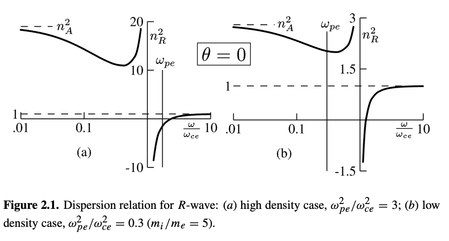
R-wave #

The R and L waves decouple because of the chirality of the circular motion of the charges, and because particles have an asymmetric response to the magnetic field due to their charge-to-mass ratios.

The R-wave is the solution \( n^2 = R \)

These are electromagnetic waves with right-handed polarization propagating along \( \vec B \)

For an electron-ion plasma,

So R-wave resonance happens when \( \omega = \omega_{c, e} \). We get electron resonance with the R-wave because electrons orbit \( \vec B \) counter-clockwise.

Cut-offs for the R wave are \[n_R ^2 = R = 0 \rightarrow \omega_R = 0\] \[\omega_R = \frac{\omega_{c, e} - \omega_{c, i}}{2} + \left( \left(\frac{\omega_{c, e} + \omega_{c, i}}{2} \right)^2 + \omega_p ^2 \right)^{1/2}\] In the strongly magnetized limit \( \omega_p / \omega_c \ll 1 \) \[\omega_R \approx \omega_{c, e} \left( 1 + \frac{\omega_{p, e}^2}{\omega_{c, e}^2} \right) \approx \omega_{c, e} \quad \text{(low-density R-wave cutoff)}\] In the un-magnetized limit \( \omega_p / \omega _c \gg 1 \) \[\omega_R \approx \omega_{p, e} + \frac{1}{2} \omega_{c, e} \approx \omega_{p, e} \quad \text{(high-density R-wave cutoff)}\]

Consider the high-frequency and low-frequency limits to get a feel for the situation:

\[\omega \rightarrow 0 \quad \rightarrow \quad n_R ^2 \approx 1 + \frac{\omega_{p, i}^2}{\omega_{c, i} ^2} \quad \text{(MHD limit)}\] \[\omega \rightarrow \infty \quad \rightarrow \quad n_R ^2 \approx 1 - \frac{\omega_{p, e}^2}{\omega^2} \quad \text{(ordinary wave)}\]

We see that low-frequency R-waves elicit a MHD response.

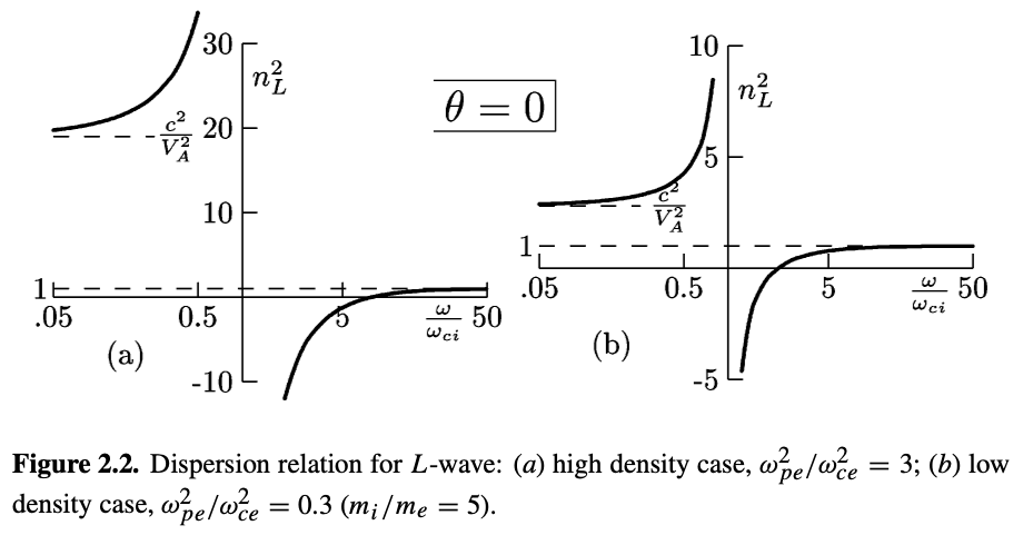
L-wave #

These are electromagnetic waves with left-handed polarization propagating along \( \vec B \)

Repeating the same process for L-waves, \( n_L ^2 - L = 0 \) we get \[n_L ^2 = 1 - \frac{\omega_{p, e}^2}{\omega(\omega - |\omega_{c, i}|)} - \frac{\omega_{p, i}^2}{\omega(\omega + |\omega_{c, e}|)}\]

The resonance condition is \( \omega = \omega_{c, i} \) because positively charged ions orbit clockwise with respect to the magnetic field.

Cut-off happens when \[\omega_L = \frac{\omega_{c, i} - \omega_{c, e}}{2} + \left[ \left(\frac{\omega_{c, i} + \omega_{c, e}}{2}\right)^2 + \omega_p ^2 \right]^{1/2}\]

The limits for the L-wave are:

• Low density: \( \omega_L \approx \omega_{c, i} (1 + \frac{\omega_{p, i}^2}{\omega_{c, i}^2}) \approx \omega_{c, i} \)
• High density: \( \omega_L \approx \omega_{p, e} - \frac{1}{2} \omega_{c, e} \approx \omega_{p, e} \)
• Low frequency: \( n_L ^2 \approx n_R ^2 \approx 1 + \frac{\omega_{p, i}^2}{\omega_{c, i}^2} \)
• High frequency: \( n_L ^2 \approx n_R ^2 \approx 1 - \frac{\omega_{p, e}^2}{\omega^2} \)

Principal Solutions - Perpendicular Propagation #

\[\theta = \pi / 2 \qquad \vec k \perp \vec B_0\] \[\rightarrow (S n^2 - RL) (n^2 - P) = 0\] There are two types of solution for waves propagating perpendicular to the magnetic field:

1. \( n^2 - P = 0 \) \[\rightarrow 1 - \frac{c^2 k^2}{\omega^2} - \frac{\omega_p ^2}{\omega^2} = 0\] This is the ordinary wave, propagating perpendicular to the magnetic field (O-wave). The refractive index does not depend on \( B_0 \) at all.
2. \( n^2 - \frac{RL}{S} = 0 \) This is a much more complicated expression, leading us to the extraordinary wave (X-wave). It has two different resonances.

Ordinary Wave (O-wave) #

Ordinary Wave

\[n_O ^2 = P = 1 - \frac{\omega_{pe}^2}{\omega ^2} - \frac{\omega_{pi}^2}{\omega^2} = 1 - \frac{\omega_p}{\omega ^2}\] \[\rightarrow 1 - \frac{c^2 k^2}{\omega^2} - \frac{\omega_p ^2}{\omega^2} = 0\]

For \( \theta = \pi / 2 \), because \( \vec E \) can be either parallel or perpendicular to the cyclotron orbits, we get hybrid oscillations. First, look at the ordinary plasma wave with \( \vec E \) linear polarized in the direction of \( \vec B \).

The resonance condition here is \( v_\phi > c \), which doesn’t happen, so there aren’t any resonances. The cut-off condition is \( \omega_O = \omega_p \) for the ordinary wave. There is no propagation below \( \omega_p \)

Extraordinary Wave (X-wave) #

X-wave

\[n_X ^2 = \frac{RL}{S}\]

We can factor the dispersion relation for the X-wave like this:

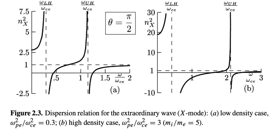
We can immediately see that the orbits are going to be complicated. With everything nicely factored, we look for resonances and cutoffs

X-wave Resonances #

The condition for resonance is:

\[(\omega ^2 - \omega_{c, i}^2)(\omega^2 - \omega_{c, e}^2) + \omega_p ^2(\omega_{c, e} \omega_{c, i} - \omega^2) \rightarrow 0\] \[\omega^2 = \frac{\omega_{u, e}^2 + \omega_{u, i}^2}{2} \pm \left[ \left( \frac{\omega_{u, e} - \omega_{u, i}}{2}\right)^2 + \omega_{p, e}^2 \omega_{p, i}^2 \right]^{1/2}\] where we define the upper hybrid frequency \[\omega_{u, \alpha}^2 \equiv \omega_{p, \alpha}^2 + \omega_{c, \alpha}^2\] Approximating the exact solutions by disregarding terms that are small in the electron/ion mass ratio, we get two resonances of the extraordinary wave \[\omega_{UH}^2 \equiv \omega_{p, e}^2 + \omega_{c, e}^2 \quad \text{Upper-hybrid X-wave}\] \[\omega_{LH}^2 \equiv \omega_{c, e} \omega_{c, i} \frac{\omega_{p, e}^2 + \omega_{c, e} \omega_{c, i}}{\omega_{p, e}^2 + \omega_{c, e}^2} \approx \omega_{c, e} \omega_{c, i} \quad \text{Lower-hybrid X-wave}\]

The resonances of the X-wave are approximately at the norm (upper hybrid) and geometric mean (lower hybrid) of the electron frequencies.

Lower Hybrid Resonance #

If we just look at the lower hybrid resonance, let’s take a look at how the currents resulting from the wave flow:

For the lower-hybrid resonance, we get \( E_y = 0 \).

From the conductivity tensor \( \sigma \), we can convince ourselves that \( |\sigma_{xx}| \ll |\sigma_{xy}| \), and

\[J_x = \sigma_{xx} E_x + \sigma_{xy} E_y \approx 0\] \[J_y = - \sigma_{xy} E_x + \sigma_{xx} E_y \neq 0\]

Interestingly, the majority of the resulting current is in the \( y \) direction, but the electric field is in the \( x \) direction.

From dispersion relation

\[J_x = \sigma_{xx} E_x + \sigma_{xy} E_y \approx 0\] \[J_y = - \sigma_{xy} E_x + \sigma_{xx} E_y \neq 0\]

From the Fourier transform of the electron momentum equation,

\[-i \omega_{LH} \vec v_e = - \frac{e}{m_e} ( \vec E + \vec v_e \cross \vec B_0) = - \frac{e}{m_e} (\vec E - \omega_{ce} \vec v_e \cross \vu z)\] We can split this in the x- and y-directions, to become \[-i \omega_{LH} v_{ex} = - \frac{e}{m_e} E_x - \omega_{ce} v_{ey} \quad \text{(x-direction)}\] \[-i \omega_{LH} v_{ey} = - \omega_{ce} v_{ex} \quad \text{(y-direction)}\]

Just from the second equation, we get

We can deduce that the y-component of displacement is much greater than the x-component

Looking at the Fourier transform of the ion equation,

In the x-direction:

In the y-direction

If we consider the various magnitudes of the frequencies and mass ratios involved, we can assume that

Combining the system of equations for the ion momentum equation, we get

\[i \left( \frac{\omega_{ci}^2}{\omega_{LH}^2} - 1 \right) v_{i x} = \frac{1}{\omega_{LH}} \frac{e E_x}{m_i}\] \[\rightarrow v_{ix} = \frac{i}{\omega_{LH}} \frac{e E_x}{m_i}\]

Then \[\left| \frac{v_{iy}}{v_{ix}} \right| = \left| - i\frac{\omega_{ci}}{\omega_{LH}} \right| \ll 1\]

So, for the ions, following the same logic as with the electrons, we have

If we compare the ion and electron velocities,

\[\frac{v_{ex}}{v_{ix}} = \frac{\omega_{LH}^2}{\omega_{ce} ^2} \frac{m_i}{m_e} \sim \frac{\omega_{ce} \omega_{ci}}{\omega_{ci}^2} \frac{m_i}{m_e} \sim \frac{\omega_{ci}}{\omega_{ce}} \frac{m_i}{m_e}\] \[= \frac{m_e}{m_i} \frac{m_i}{m_e} = 1\]

So the x-components of the ion and electron currents have the same magnitude and cancel each other out.

The upper hybrid resonance produces a similar effect, but the frequency of the upper hybrid resonance is higher.

Upper Hybrid Resonance #

Same equations of motion, and same dispersion relationship as before, but with a different frequency

so when we consider the UH resonance, we consider the ions to be essentially stationary.

Using \( \omega_{UH}^2 = \omega_{pe}^2 + \omega_{ce}^2 \)

Again from the conductivity tensor,

\[J_x = \sigma_{xx} E_x + \sigma_{xy} E_y \approx 0\] \[J_y = - \sigma_{xy} E_x + \sigma_{xx} E_y \neq 0\]

\[J_x = i \omega_{UH} \epsilon_0 E_x\] \[J_y = - \omega_{ce} \epsilon_0 E_x\]

The displacement current \( \epsilon_0 \pdv{\vec E}{t} \) is

This is the negative of the electron current \( J_x \), so the two cancel out. Again we get \( J_x = 0 \) but \( J_y \neq 0 \).

X-wave Cutoff #

Cut-offs of the extraordinary wave correspond with roots of the numerator \[\omega_X = \left[ \left(\frac{\omega_{c, e} + \omega_{c, i}}{2} \right)^2 + \omega_p ^2 \right] ^{1/2} \pm \frac{\omega_{p, e} - \omega_{c, i}}{2}\]

• High-density: \( \omega_X \rightarrow \omega_{p, e} \pm \frac{1}{2} \omega_{c, e} \)
• Low-density: \( \omega_X \rightarrow \omega_{ce} (1 + \frac{\omega_{p, e}^2}{\omega_{c, e}^2}) \) and \( \omega_{c, i} (1 + \frac{\omega_{c, e}}{\omega_{c, i}} \frac{\omega_{p, e}^2}{\omega_{c, e}^2}) \)
• Low-frequency: \( n_X = 1 + \frac{\omega_{p, i}^2}{\omega_{c, i}^2} \)
• High-frequency: \( n_X^2 = 1 \), same as the free-space wave, so the plasma is transparent.

Overdense and Underdense Plasmas #

Take a look at the “sum” terms in the dispersion relation

\[S = \frac{1}{2} (R + L) = 1 - \sum_\alpha \frac{\omega_{p, \alpha}^2}{\omega^2 - \omega_{c, \alpha}^2}\] \( \omega \) has units of radians per second, so the timescale of this term is un-normalized. Because there are two different characteristic frequencies \( \omega_p \) and \( \omega_c \), we can’t normalize to one of them. Let’s choose to normalize to the cyclotron frequency, \( \omega / \omega_{c, \alpha} \). Then we can write \( S \) as \[S = 1 - \sum _\alpha \frac{\omega_{p, \alpha ^2}}{\omega^2} \frac{1}{(\omega / \omega_{c, \alpha})^2 - 1}\] The term \( (\omega_{p, \alpha} / \omega_{c, \alpha})^2 \) is an important characteristic for a magnetized plasma. Writing out the definitions of each, \[\frac{\omega_{p, \alpha}^2}{\omega_{c, \alpha}^2} = \frac{\frac{n_\alpha q_\alpha ^2}{\epsilon_0 m_\alpha}}{\frac{q_\alpha ^2 B_0 ^2}{m_\alpha ^2}} = \frac{n_\alpha m_\alpha}{\epsilon_0 B_0 ^2} = \frac{c^2}{v_{A, \alpha} ^2}\] where the Alfven velocity \( v_{A, \alpha} \) is \[v_{A, \alpha} ^2 = \frac{B_0 ^2}{\mu_0 n_\alpha m_\alpha}\] So the ratio of the plasma frequency to the cyclotron frequency is \[\frac{\omega_{p, \alpha}^2}{\omega_{c, \alpha}^2} \sim \frac{n}{B_0 ^2} \sim \frac{\text{mass density of charges}}{\text{energy density of magnetic flux}}\] or, equivalently \[\frac{\omega_{p, \alpha}^2}{\omega_{c, \alpha}^2} \sim \frac{c^2}{v_{A, \alpha} ^2} \sim \frac{(\text{velocity in free space})^2}{(\text{speed of magnetic perturbations})^2}\] We have two interpretations of the parameter. It measures density vs. magnetization, and is also like a refractive index for magnetic perturbations.

• If \( \omega_p < \omega_c \), we have an “under-dense” plasma. Density is low enough relative to magnetization that the response is dominated by magnetization.
• If \( \omega_p > \omega_c \), we have an “over-dense” plasma. It is weakly magnetized.

Generally speaking, over-dense plasmas are more unstable than under-dense plasmas. It’s easier to keep under-dense, well magnetized plasmas in thermal nonequilibrium for longer periods of time.

Fast and Slow Waves & Birefringence #

Our dispersion relation looks something like \[n^2 = \frac{B \pm F}{2A} \qquad n ^2 = n^2(\omega, \theta)\]

where the descriminant \( F \) is positive-definite. This means that for any angle \( \theta \) we get two solutions \[n_1 ^2 = \frac{B + F}{2A} \qquad n_2 ^2 = \frac{B - F}{2A} \sim \frac{c^2}{v_\phi ^2}\] We’ll end up with “fast” waves with higher \( v_\phi \) and “slow” waves.

All anisotropic media exhibit fast and slow waves, as a general property. Because there are two indices of refraction, we call the material birefringent. Light entering a birefringent material will be split and exit in two locations.

There are many parallels between magnetized plasma and birefringent crystals, but there are some important differences

• A plasma can have a moving optical axis
• Birefringent properties of plasma are strong functions of density and magnetic field
• There is a strong thermal response to the index of refraction, leading to e.g. Langmuir waves

Despite these differences, there is a strong analogy between the cold plasma dispersion relation and the theory of birefringent crystals.

Wave Normal Surfaces #

Defined as the “locus of phase velocity vectors, \( \vec v_{\phi} = \frac{\omega}{k} \vu k \)” (Stix). Since the axis of symmetry for a cold magnetized plasma is the direction of the magnetic field, this is really just a polar plot of \( v_\phi \) and \( \theta \), the angle between \( \vec k \) and \( \vec B \)

The cold plasma dispersion relation gave us

\[A n^4 - B n^2 + C = 0 \] \[A = S \sin ^2 \theta + P \cos ^2 \theta\] \[B = R L \sin ^2 \theta + P S (1 + \cos ^2 \theta)\] \[C = PRL\] Solving the quadratic, we get \[n^2 = \frac{B \pm F}{2A} \qquad F^2 = B^2 - 4AC = (RL - PS)^2 \sin^4 \theta + 4 P^2 D^2 \cos ^2 \theta\]

If we define \( u = v_\phi / c = 1 / n \), then this becomes

(this doesn’t work where there’s a cut-off where \( v_\phi = 0 \)). Note that the \( \theta \) dependence of \( A \), \( B \), and \( C \) only depends on \( \sin ^2 \theta \) and \( \cos ^2 \theta \) terms. Therefore

and

\[u ( \pi / 2 - \theta) = u(\theta - \pi / 2)\] So, the surfaces formed by \( u \) are symmetric about \( \theta = 0 \) and \( \theta = \pi / 2 \).

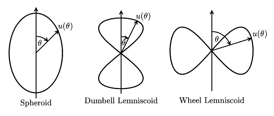
There are three topographical types of wave normal surfaces:

We really only care about the topographical properties of the wave normal surface, since the topographical properties remain unchanged within a region of the CMA diagram. The exact values aren’t nearly as useful.

Spheroid #

If \( P \) and \( S \) have the same sign, then \( u \neq 0 \) everywhere in the volume. Since \( u \) can not go to \( \infty \) within the volume, \( u \) must be real everywhere. Topographically, this is a spheroid. We don’t make any distinction between prolate and oblate spheroids; spheroids simply have a real, non-zero \( u \) for every angle \( \theta \).

Example: fast and slow waves

Applying the approximation \( \omega_{ci} \ll \omega_{ce} \)

Since \( u_R > u_L \) everywhere in the region, the wave normal surfaces will be nested spheroids with the R-wave surface surrounding the L-wave surface.

Lemniscoids #

If \( P/S < 0 \), then at least one branch has \( u \rightarrow 0 \) at the resonance angle \( \theta_{res} \) and its complement at all points within the volume. The cross generated near \( u = 0 \) by these angles when rotated about the axis of symmetry forms a pair of cones touching vertex to vertex. If \( u \) is real inside the cone, then the wave normal surface is a dumbbell lemniscoid. If it is real outside the cone, then we have a wheel lemniscoid.

Wave normal surfaces are not allowed to intersect, since two solutions to the dispersion relation can only coincide at \( \theta = 0 \) or \( \theta = \pi / 2 \). In general, there are two solutions for \( u \). If \( P / S > 0 \), then there can only be spheroids.

If we examine the dispersion relation in the vicinity of a resonance \( \theta_{res} \) where \( A = 0 \), we can eliminate the \( n^4 \) term in the dispersion relation and get the remaining solution

where we’ve used \( \sin ^2 \theta \sim (- P / S) \cos ^2 \theta \). The solution is nonzero within any volume, so it represents a spheroid. If \( P / S < 0 \), then the second solution, if it has a real \( u \), is a spheroid. Again, because the wave normal surfaces are not allowed to intersect, the spheroid must enclose the lemniscoid.

CMA Diagram #

We can finally trace out all of the surfaces defined by our cut-offs and resonances in a CMA diagram:

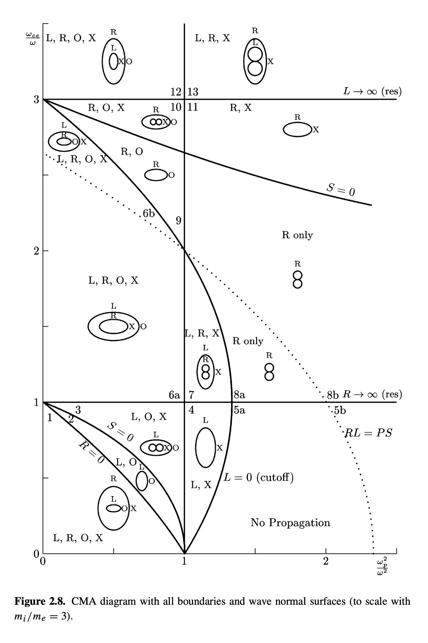
Each line is a cutoff or resonance, except the line at \( RL = PS \) where the O and X waves both follow the plasma relation \( n^2 = P \). We can fill in the diagram with wave-normal surfaces which encode the possibility of information transfer. If a wave can’t propagate due to cut-off or bandgap, it becomes invisible.

• Inside any volume bounded by cutoff/resonance curves (BV) there are no cutoffs
• If there is a resonance \( n \rightarrow \infty \) inside a bounded volume, then everywhere else in that bounded volume there exist resonance angles \( \theta \) corresponding to the same resonance. That is because \( P / S \) can not change sign within a bounded volume.
• For any angle \( \theta \) where \( n \neq 0 \) or \( \infty \), then only one branch will be either real or imaginary. There is no transition from cut-off to not-cut-off
• The wave normal surface is symmetric about the magnetic axis and \( \theta = \pi/2 \)
• Classes of solutions can only coincide where \( \theta = 0, \pi/2 \) or \( RL = PS \), where the O, L, and R waves have equivalent dispersion .

There are three topological possibilities for wave-normal surfaces in the CMA diagram.

1. \( v_\phi \neq 0 \) for all angles \( \theta \) (wave exists for all \( \theta \)). Then the wave-normal diagram is roughly spherical
2. \( P / S < 0> \), so there is a solution \( \tan ^2 \theta = - P / S \). Then the resonance angle defines a cone about the magnetic axis. Propagation will either be allowed everywhere inside the cone, or everywhere outside the cone.

When we talk about locations in the CMA diagram, we usually use the Altar-Appleton factors \( X \) and \( Y \)

\[R = 1 - \frac{X}{Y + \mu} + \frac{X}{Y - 1}\] \[L = 1 + \frac{X}{Y - \mu} - \frac{X}{Y + 1}\]

where

\[X = \frac{\omega_{pe}^2}{\omega ^2}\] \[Y = \frac{\omega_{ce}}{\omega}\] \[\mu = \frac{m_i}{Z m_e}\]

Phase and Group Velocities #

Ordinary plasma wave

\[v_g = \left. \pdv{\omega}{k} \right|_{k_0}\]

where \( k_0 \) is the center of a wave group in space

\[v_\phi = \frac{\omega}{k}\]

For the O-waves,

\[n^2 = 1 - \frac{\omega_p ^2}{\omega^2} = \frac{c^2 k^2}{\omega^2}\] \[\rightarrow \omega ^2 = \omega_p ^2 + c^2 k^2\]

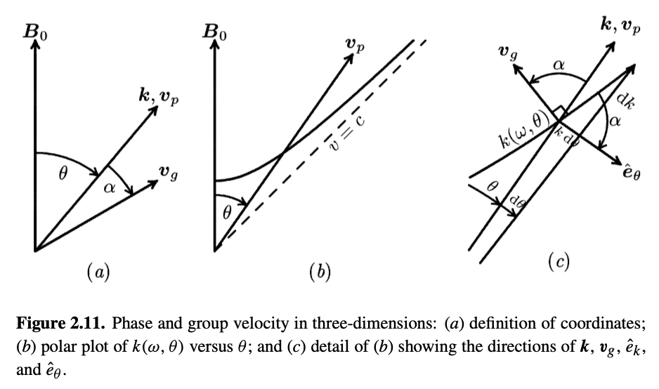
In 3 dimensions, the group velocity can be in a different direction than the phase velocity

We define \( \alpha \) to be the angle between the phase and group velocities, then

From Swanson, we can express \( \alpha \) in terms of the refractive index:

\( \alpha \) helps us identify the relationship between \( v_\phi \) and \( v_g \). For example, in a spheroid wave normal surface, there is no variation of \( \vec k \) with \( \theta \), so \( \tan \alpha = 0 \) and \( \vec v_\phi \) and \( \vec v_g \) are in the same direction.

But, if you have any variation with \( k \) with \( \theta \), then \( \vu v_\phi \) and \( \vu v_g \) are not identical.

Whistler Waves #

Whistler waves emit in partially magnetized plasma, where

If we look at the R-wave dispersion relationship, we find the phase and group velocities are

But the phase velocity is

and the group velocity is exactly twice the phase velocity

Propagation of Whistler Waves #

To see the direction of the group velocity for Whistler waves, we consider the approximate dispersion relation for an arbitrary propagation angle \( \theta \), in the intermediate frequency range \( \omega_{ci} \ll \omega \ll \omega_{ce} \sim \omega_{pe} \),

So roughly, we have an ordering

Because \( P \) is so much larger, any \( E_z \) will dominate the behavior, and we will just get the behavior of an electrostatic wave, so we let \( E_z \rightarrow 0 \) and consider just the x-y behavior:

If \( \theta \neq \pi / 2 \), noting that \( |S| \ll |D| \) it reduces to

Using \( n = c / (\omega / k) \) and \( D = \omega_{pe}^2/(\omega \omega_{ce}) \),

\[\frac{\omega_{pe}^2}{\omega \omega_{ce}} = \frac{c^2 k^2}{\omega ^2} \cos \theta\] \[\omega = \frac{k^2 c^2 \omega_{ce} \cos \theta}{\omega_{pe}^2}\]

If \( \theta = 0 \) (parallel propagation), then this is the generic R-wave propagation.

The angle for the group’s velocity is given by

This tells us that \( \alpha \) is negative, so the direction of the group velocity \( \vec v_g \) always lies between \( \vec B \) and \( \vec v_\phi \). The angle between \( \vec B \) and \( \vec v_g \) is then

We can find the maximum angle \( \theta + \alpha \) between the group velocity and \( \vec B \) by differentiating, to find that the maximum angle is when \( \tan ^2 \theta = 2 \), so

\[\tan (\theta + \alpha)_{max} = \frac{\tan \theta}{2 + \tan ^2 \theta} = \frac{\sqrt{2}}{2 + 2} = \frac{1}{\sqrt{8}}\] \[(\theta + \alpha)_{max} = \tan ^{-1} \frac{1}{\sqrt{8}} = 19.5 ^{\circ}\]

This means that there is a 19-degree cone of propagation around the direction of \( \vec B \) where whistler modes can propagate.

Faraday Rotation #

A linearly-polarized electromagnetic wave can be written as a sum of left-handed and right-handed circularly polarized waves.

\[E_R = (E_{Rx}, E_{Ry}) = \hat E(e^{i \theta}, e^{i \theta} e^{i \pi / 2}) = \hat E e^{i \theta} (1, i)\] \[E_L = (E_{Lx}, E_{Ly}) = \hat E(e^{i \theta}, e^{i \theta} e^{-i \pi / 2}) = \hat E e^{i \theta}(1, -i)\]

This is a useful decomposition when we consider linearly polarized light propagating in a magnetized medium, because in a plasma the left- and right-handed polarized components are Faraday rotated in different directions, and a phase difference adds up as the wave propagates through a plasma.

For a wave propagating through a magnetized plasma parallel to the magnetic field (\( \theta = 0 \)), the Faraday rotation caused by the difference in refractive index between the R- and L-wave modes.

Let’s work out the math to see how that happens. Writing out the Fourier representation of our superposition: \[E_R = \hat E e^{i (k_R z - \omega t)} \qquad E_L = \hat E e^{i (k_L z - \omega t)}\] \[E = E_R + E_L\] \[\text{Re}(E) = \hat {E} [\cos \phi_R + \cos \phi_L]\] \[= \hat E \left[2 \cos \frac{\Delta \phi}{2} \cos \frac{\overline{\phi}}{2} \right]\]

where \( \phi_R = k_R z - \omega t \), \( \phi_L = k_L z - \omega t \), \( \Delta \phi = \phi_R - \phi_L \), and \( \overline{\phi} = \frac{\phi_R + \phi_L}{2} \)

\[\pdv{}{z} (\Delta \phi) = \pdv{}{z} \left( \frac{\omega}{c} \frac{(n_L - n_R)}{2} z \right)\] \[ = \frac{\omega}{2c} \Delta n\]

For high-frequency waves, the refractive index difference between left- and right-handed modes is

\[\Delta n = \frac{\omega_{pe}^2}{\omega ^2} \frac{\omega_{ce}}{\omega}\] \[\pdv{\Delta \phi}{z} = \frac{1}{2c} \frac{\omega_{pe}^2 \omega_{ce}}{\omega ^2} \propto \lambda ^2 n_e B_0\]

The amount of polarization rotation (chord-integrated along the length of propagation) of a laser of known frequency gives a measurement of the product \( n_e B_0 \). If you know one, and \( B \) is high enough, you can find the other from Faraday rotation.

Plasma Interferometry #

We can measure the plasma density by transmitting O-waves through the plasma, and measuring the resulting phase change.

We transmit some signal through the plasma \( S_p = A_p e^{i (\phi_p - \omega t)} \)

and also send a reference signal to the same receiver

We add the resulting beams and measure the signal \( S \):

In vacuum, we set \( S = 0 \) by matching the phases of the reference and transmitted signals with \( A_P = - A_R = A \) and \( \phi_P = \phi_0 = \phi_R \)

Now, if we have a plasma, the phase change

\[\Delta \phi(t) = \int _0 ^L k_z (z, t) \dd z - \int _0 ^L k_0 \dd z\] \[= \frac{\omega}{c} \int _0 ^L (n - 1) \dd z\]

Within the plasma, \( n^2 = n_O ^2 = P = 1 - \frac{\omega_p ^2}{\omega ^2} \)

At the detector, we measure

\[S = A (e^{i \Delta \phi} - 1) e^{i (\phi_0 - \omega t)}\] \[= 2 i \sin \frac{\Delta \phi}{2} e^{i \Delta \phi / 2} e^{i (\phi_0 - \omega t)}\]

The actual measurement we’re going to be able to get our of our instrument is the energy deposited by the signal, which is \( |S^2| \)

High-Frequency Interferometry #

When the wave frequency is much higher than the plasma frequency, which the usual case when either optical or infrared waves are used, then we can expand the square root

\[\Delta \phi = - \frac{\omega}{c} \int _{0} ^{L} (1 - \frac{1}{2} \frac{\omega_p ^2}{\omega ^2} - 1) \dd z\] \[ = - \frac{1}{2 \omega c} \int _0 ^L \omega _p ^2 \dd z \propto n_e \lambda L\]