Quasi-Linear Theory#
(Goldston and Rutherford, Chapter 25 is a good reference)
From kinetic theory, we saw that instabilities can develop when a wave is resonant with particles in an appropriate region of the velocity distribution function. This is essentially the reverse of Landau damping (“inverse Landau damping”).
We saw an example of the “bump-on-tail” instability, where we have a distribution where there is a high-energy population that causes \( \partial f / \partial v \) to be positive for certain values of \( \omega / k \). This is a generalization of the 2-stream instability.
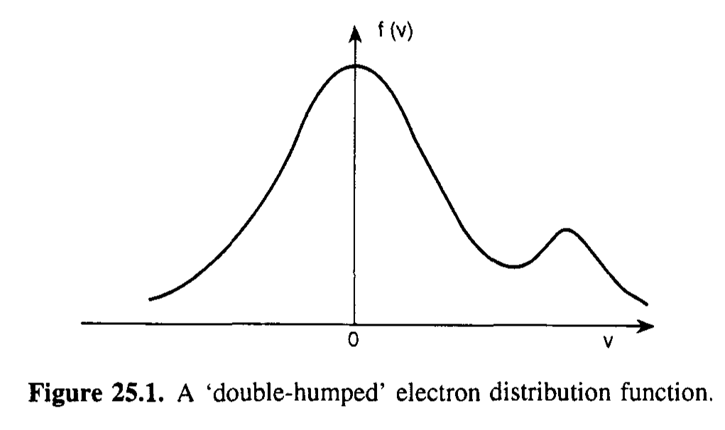
If \( \omega \approx \omega_p \) (Langmuir oscillations), then \( k \) governs \( v_\phi \). If, for certain values of \( k \), \( \pdv{f}{v} > 0 \), then that \( v_\phi \) can excite an unstable mode.
So far, when looking at things through the lens of linear theory, we have assumed that any perturbation is very small. This allowed us to represent perturbations spatially as Fourier modes, superimpose different modes, and to actually solve the Vlasov equations.
But linear theory predicts exponential growth terms \( e^{\omega_i t} \) for \( \omega_i > 0 \). In that case, we quickly step away from the “small perturbation” assumption into a different region. That doesn’t really happen in real-world plasmas. In reality, non-linear effects limit the amplitude growth.
These nonlinear effects are generally divided into two categories: wave-particle interactions and wave-wave interactions.
Wave-particle interactions include situations like particle trapping, warm interactions.
Wave-wave interactions occur if the wave amplitude grows so large that amplitudes of different waves are able to interact with each other. These are pretty complicated, and mostly out of scope of this class, and are covered in texts like Sagdeev and Galeev.
Assumptions of Quasi-Linear Theory#
- Amplitudes of wave modes are still small enough that linear assumptions about structure, frequency and instantaneous growth are valid
- Wave spectrum is dense enough for decoherence between modes
- Damping and growth are much less than the real component of frequency
- Saturation of the instability occurs before wave-wave interactions become significant
Theoretical Framework#
To derive the quasi-linear process, we go through the same process as before. We consider the Vlasov equation in 1D
\[\pdv{f}{t} + v \pdv{f}{x} - \frac{e}{m} E \pdv{f}{v} = 0\]Previously, we linearized by assuming
\[f(x, v, t) = f_0 (v) + \tilde{f}_1 (v) e^{- i (\omega t - k x)}\] \[E(x, t) = 0 + \tilde{E} e^{-i (\omega t - k x)}\]Then, linearized Vlasov becomes
\[- i (\omega - kv) f_1 = \frac{e}{m} E \pdv{f_0}{v}\]Now, we consider a “slow” evolution of \( f_0 \), rather than just having an unchanged initial state \( f_0 \). We then write \( f_0 \) as the spatially averaged (over many wavelengths) part of the complete distribution function
\[f(x, v, t) = f_0 (v, t) + f_1 (x, v, t)\] \[f_1 (x, v, t) = \sum_k \tilde{f}_{1k} (v) e^{i (kx - \omega t)}\] \[E(x, t) = \sum_k \tilde{E}_k e^{i (kx - \omega t)}\]
The spatially averaged Vlasov equation becomes:
\[\pdv{f_0}{t} = \frac{e}{m} \langle E \pdv{f_1}{v} \rangle\]Noting that
\[\langle \vec A \cdot \vec B \rangle = \frac{1}{2} \text{Re} \left[ \vec A \cdot \vec B ^\star \right]\] \[\pdv{f_0}{t} = \frac{e}{2m} \text{Re} \left[ \sum_k E_x ^\star \pdv{f_{1k}}{v} \right]\]If \( f_0 \) evolves slowly, it can be treated as essentially constant in time with respect to \( f_1\). So we can use the \( f_1 \) value from the linearized Vlasov equation:
\[f_{1k} = \frac{i e \tilde{E}_k}{m} \frac{\partial f_0 / \partial v}{\omega - k v}\] \[\pdv{f_0}{t} = - \frac{e^2}{2 m^2} \pdv{}{v} \left[ \text{Im} \left( \sum_ik | \tilde{E}_k|^2 \frac{1}{\omega - k v} \right) \pdv{f_0}{v}\right]\]If we define \( \omega = \omega_r + i \gamma \approx \omega_k + i \gamma _k \):
\[\pdv{f_0}{t} = \frac{e^2}{2 m^2} \pdv{}{v} \left[ \sum_ik | \tilde{E}_k|^2 \frac{\gamma_k}{(\omega_k - k v)^2 + \gamma_k ^2} \pdv{f_0}{v} \right]\]If the available \( k \) modes are dense enough, we can convert the sum to an integral. The spectral energy density of the E-field is
\[\frac{\epsilon_0}{2} \sum_k | \tilde{E}_k|^2 \rightarrow 2 \int _{-\infty} ^{\infty} \mathcal{E}(k) \dd k\]Also, for very small \( \gamma_k \):
\[\frac{\gamma_k}{(\omega_k - k v)^2 + v_k^2} \rightarrow \pi \delta(\omega_k - k v)\]Then
\[\pdv{f_0}{t} = \frac{2 \pi e^2}{\epsilon_0 m^2} \pdv{}{v} \left[ \pdv{f_0}{v} \int _{-\infty} ^{\infty} \mathcal{E}(k) \delta(\omega_k - k v) \right]\]This is similar to a diffusion equation in velocity space \[T_t = \kappa \grad ^2 T + f\]
We’ve got \[\pdv{f_0}{t} = \pdv{}{v} \left( D(v) \pdv{f_0}{v} \right)\]
where
\[D(v) = \frac{2 \pi e^2}{\epsilon_0 m^2} \int _{-\infty} ^{\infty} \mathcal{E}(k) \delta(\omega_k - k v) \dd k\] \[= \frac{2 \pi e^2}{\epsilon_0 m^2 v} \mathcal{E}(\omega / v)\]
In this context, if \( \gamma > 0 \) then the distribution \( f_0 \) will “diffuse” in velocity-space near the \( v_\phi \) where instability develops. Remember that the particles will be conserved in space, this gives us an intuition how the distribution will “flatten out” whenever there is a region of instability. It must “diffuse” outwards from the instability, and tend toward a marginally stable “flat” distribution.
If we integrate in time, as \( t \rightarrow \infty \) the long-term behavior is
\[\mathcal{E}(k) = \frac{m \omega ^2}{2 k^3} \int _{v_1} ^{v = \omega / k}[ f_0 (v, \infty) - f_0 (v, 0)] \dd v\]when \( v_1 \) and \( v_2 \) can be determined from particle conservation
\[\int _{v_1} ^{v_2} f_0 (v, \infty) \dd v = \int _{v_1} ^{v_2} f_0 (v, 0) \dd v\]Wave Saturation due to Finite Amplitude Effects#
Particle trapping due to certain wave amplitudes can influence collisionless damping and growth.
The important time scales for particle trapping are:
\( \tau_B = \sqrt{\frac{m_e}{e k E_0}} \) is the electron bounce period.
\( \tau_p = 1 / \omega_p = \sqrt{\frac{\epsilon_0 m_e}{n_0 e^2}} \) is the plasma period.
\( \tau_L = (\gamma_L)^{-1} \) is the Landau damping time scale. If the Landau damping is much smaller than the bounce period, then you don’t really see the trapping.
Trapped particles are significant for \( \tau_L \gg \tau_B \gg \tau_p \).
The general analysis approach (from Swanson) for particle trapping is:
- Start with the Vlasov equation
- Use the trapped particle equation of motion
- Use conservation of wave and particle energy
The end result is \( \gamma = \gamma(t, \tau_B, \tau_L) \).