Plasma Models #

Working towards MHD #

Let’s start from a full-particle description with the goal of reaching a continuum description (kinetic model). Then, we’ll look at the forces on the separate species and form a multi-fluid model, finally simplifying to a single-fluid MHD model.

The most important question to ask ourselves is “when is this model going to be useful?” The MHD model is the mathematical model for magnetized plasmas that are treated as a fluid. This means that we can define a fluid element (some lil’ box of plasma) and define the physical properties (mass, density, magnetization, etc.) of the element. We need to make some assumptions about scale in order to do this. In terms of spatial scales, we abstract properties below a discrete scale \( a_0 \) into the properties of a fluid element

Length scales smaller than the discrete scale will not be properly captured by the model, so scales like the particle radius will be meaningless in our fluid model.

Plasma Definition #

A plasma is a quasi-neutral gas of charged and neutral particles which exhibit collective behavior. The particles (electrons, ions, neutrals) interact through EM fields and collisions.

Mathematically you would think that plasmas could be treated as individual particles. Doing so gives an N-body problem with classical interactions through the Lorentz force (Coulomb interaction removed by assumption of quasi-neutrality) and binary collisions. Each particle \( i \) has a well-defined mass \( m_i \) and charge \( q_i \) which do not change in time. The governing equations are

\[\dv{\vec v_i}{t} = \frac{q_i}{m_i} (\vec E + \vec v_i \cross \vec B) + \sum_{j \neq i} \left[ \left. \dv{\vec v_{ij}}{t} \right|_{coll} (\vec r_i - \vec r_j) \right]\] \[\dv{\vec r_i}{t} = \vec v_i\]

The fields E and B are described by the Maxwell equations

\[\pdv{B}{t} = - \curl E\] \[\frac{1}{c^2} \pdv{E}{t} = \curl B - \mu_0 \sum_i q_i v_i \delta (r - r_i)\] \[\div B = 0\] \[\epsilon_0 \div E = \sum_i q_i \delta (r - r_i)\]

Klimontovich Equation #

Re-writing the force relations as a statement of conservation in phase space, we get Klimontovich equation for species \( \alpha \)

The particle phase space is defined by \[N_\alpha(p, q) = \sum_i \delta(p - p_i) \delta(q - q_i)\] where \( p \) and \( q \) are generalized momentum and position coordinates. The resulting \( N(p) \) looks very spiky, with nonzero values only at the exact values inhabited by particles. Unfortunately, that means that only the tools of discrete mathematics are applicable to the distribution, and we’re forbidden from our favorite tool (calculus). To make the analysis possible, we can smooth over the discreteness by performing an ensemble average of the Klimontovich equation. This gives us a statistical description using smooth distribution functions:

That is, \( f(x, v, t) \) is the number of particles at position \( x \) with velocity \( v \) at time \( t \) . We also work with normalized distributions which give the probability of finding a particle.

By our definition, we can integrate to get the total number of particles at time \( t \) .

The ensemble averaging process works well if the the number of particles is very large

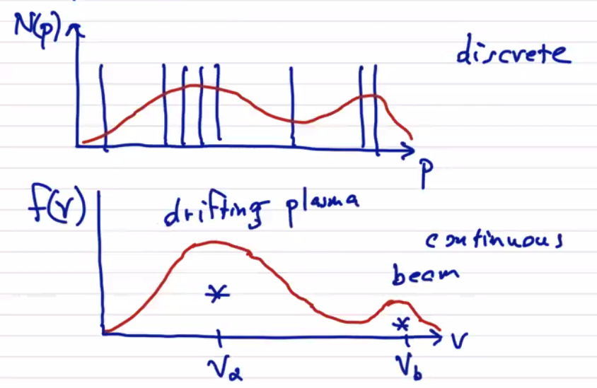
See a kinetic theory text (e.g. Krall and Trivelpiece) for a full description of the ensemble averaging process.

Now we can write our Klimontovich equation in terms of continuous quantities

The collision terms now have an infinite number of cross terms. We call this the BBGKY (Bogoliubov–Born–Green–Kirkwood–Yvon) hierarchy.

Expressing as the Boltzmann equation (generally called the Boltzmann-Maxwell equation, since the solution requires solving for the electromagnetic fields of the Maxwell equations)

We leave the collision term in. A lot of the work of kinetic theory is coming up with an applicable form of the collision operator which is appropriate but still simple enough to solve. We often write the collision operator as the product of binary collisions

Notice that the terms \( \vec v \cdot \pdv{f_\alpha}{\vec x} \) and \( \frac{q_\alpha}{m_\alpha} (\vec E + \vec v \cross \vec B) \cdot \pdv{f_\alpha}{\vec v} \) are advection equations, advecting in \( \vec x \) and \( \vec v \) respectively. If we ignore the collision term (set the RHS to zero) we have the Vlasov equation.

Note that the fields E and B at any location are generated from the charges and currents of the entire plasma volume, including externally applied fields. As a result, there’s an inherent integrating process taking into account the sources across the whole volume that leads to long-range smoothly varying forces. This is in contrast to the collisional effects, which by their nature lead to very short range abrupt forces. It makes sense to make a distinction between the long-range electromagnetic forces and the short range collisional forces.

Because the Boltzmann-Maxwell model is inherently 6-dimensional, it is a very challenging model to implement. The B-M model provides a complete description, but it is often too detailed to solve.

If we solve the Vlasov equation for two parallel opposite beams, for example, we see that the

As it turns out, the integral, centroid, and variance are all that are required to fully describe a Maxwellian distribution

In other words, we can write the Maxwellian distribution as \( f_M(n_0, \vec v_\alpha, T_\alpha ; \vec v) \) . We care about Maxwellian distributions so much in plasma physics because it is the solution to the Boltzmann equation for \( \left. \pdv{f_\alpha}{t} \right|_{coll} = 0 \) (Vlasov equation). That’s not saying that there are no collisions, it is saying that there are so many collisions that the effect is isotropic and the overall force is zero.

Another feature of the Maxwellian distribution is \( \vec v \cdot \pdv{f_\alpha}{\vec x} = 0 \) . This is a famous result called the Boltzmann H-theorem, and says that any initial distribution will relax (and very quickly) to a Maxwellian distribution.

By replacing our velocity distribution with the associated Maxwell distribution, we arrive at a Plasma Fluid Model