Two-Fluid Plasma Model (ions-electrons)#
Restricting our multi-species fluid model to ions and electrons, what can we say about wave behavior in a magnetized 2-fluid plasma? Let’s start with a cold plasma approximation ( \( p = 0 \) ) and neglect collisions. The momentum equation reduces to
\[m_\alpha \left( \pdv{\vec v_\alpha}{t} + \vec v_\alpha \cdot \grad \vec v_\alpha \right) - q_\alpha (\vec E + \vec v_\alpha \cross \vec B) = 0\]From here on out we can avoid some clutter (and wrist strain) by dropping the \( \alpha \) subscripts and acknowledging that we have sets of equations for ions and electrons. Apply a perturbation to an equilibrium \( g = g_0 + g_1 \)
\[m \left(\pdv{\vec v_0}{t} + \vec v_0 \cdot \grad \vec v_0 + \pdv{\vec v_0}{t} + \vec v_1 \cdot \grad \vec v_0 + \vec v_0 \cdot \grad \vec v_1 + \vec v_1 \cdot \grad \vec v_1 \right) \\ \qquad - q (E_0 + E_1) - q (\vec v_0 \cross \vec B_0 + \vec v_1 \cross \vec B_0 + \vec v_0 \cross \vec B_1 + \vec v_1 \cross \vec B_1) = 0\]We can drop some terms because equilibrium has to satisfy the original equation. We can balance all of the subscript-0 terms and sum them to get zero.
\[m \left( \pdv{\vec v_1}{t} + \vec v_1 \cdot \grad \vec v_0 + \vec v_0 \cdot \grad \vec v_1 + \vec v_1 \cdot \grad \vec v_1 \right) + q (- E_1 - \vec v_1 \cross \vec B_0 - \vec v_0 \cross \vec B_1 - \vec v_1 \cross \vec B_1)\]Let’s now make the assumption that the perturbation is small, that is \( g_1 \ll g_0 \) . That means that nonlinear products of perturbation terms are negligible (linearization process).
\[m \left( \pdv{\vec v_1}{t} + \vec v_0 \cdot \grad \vec v_1 + \vec v_1 \cdot \grad \vec v_0 \right) - q \vec E_1 - q (\vec v_1 \cross \vec B_0 + \vec v_0 \cross \vec B_1) = 0\]Now, assume that the equilibrium is a static equilibrium, that is \( \vec v_0 = 0 \) . If we decompose into components that are parallel and perpendicular to the equilibrium magnetic field \( \vec B_0 \) , then
\[\pdv{v_{1, \parallel}}{t} - \frac{q}{m} E_{1, \parallel} = 0\] \[\pdv{\vec v_{1, \perp}}{t} - \frac{q}{m} \left(\vec E_{1, \perp} + B_0 \vec v_{1, \perp} \cross \vu z \right) = 0\]
The parallel component \( E_{1, \parallel} \) will lead us to the ordinary wave (O-wave). Consideration of the more general case with perpendicular components will lead to the X-wave.
The plasma velocity is related to the fields through the current density (Maxwell equations). Faraday’s law gives
\[\pdv{\vec B}{t} = - \curl \vec E\] \[\rightarrow \curl \pdv{\vec B}{t} = - \curl \curl \vec E = - \grad (\div \vec E) + \nabla ^2 \vec E \]
Ampere’s law gives
\[\epsilon_0 \pdv{\vec E}{t} = \frac{1}{\mu_0} \curl \vec B - \sum_{\alpha} q_\alpha n_\alpha \vec v_\alpha\] \[\epsilon_0 \pdv{^2 \vec E }{t ^2} = \frac{1}{\mu_0} \curl \pdv{\vec B}{t} \\ = \frac{1}{\mu_0} \left[ \nabla ^2 \vec E - \grad (\div \vec E) \right] - \sum_\alpha q_\alpha \pdv{}{t} (n_\alpha \vec v_\alpha) \]
Since this is a linear system, assume that the perturbed quantities have a wave-like structure. That is, the perturbed quantities \( g_1 \) are proportional to \( e^{i(\omega t + \vec k \cdot \vec r)} \) . This lets us transform the spatial and temporal derivatives into factors of \( \omega \) and \( \vec k \)
\[- \epsilon_0 \omega ^2 \vec E_1 = - \frac{1}{\mu_0} \left[k^2 \vec E_1 - \vec k (\vec k \cdot \vec E_1) \right] + i \omega e n_0 \vec v_1\]Let’s now consider only high frequency oscillations, assuming that only the electrons respond and the ions remain stationary. There’s nothing particularly complicated about including the ion response, this just lets us drop the \( \alpha \) subscripts and focus on a single set of equations.
\[- i \omega \frac{e n_0}{\epsilon_0} \vec v_1 = (\omega ^2 - c^2 k^2) \vec E_1 + c^2 \vec k (\vec k \cdot \vec E_1)\]Now let’s apply the perturbed form to the linearized momentum equation
\[\pdv{v_{1, \parallel}}{t} - \frac{q}{m} E_{1, \parallel} = 0 \\ \rightarrow i \omega v_{1, \parallel} = - \frac{e}{m} E_{1, \parallel} \\ \rightarrow i \omega \frac{e n_0}{\epsilon_0} v_{1, \parallel} = \frac{e^2 n_0}{\epsilon_0 m} E_{1, \parallel}\]Combine the momentum equation and the Maxwell equations to eliminate \( \vec E_1 \) and \( \vec v_1 \)
\[\frac{e^2 n_0}{\epsilon_0 m} E_{1, \parallel} = ( \omega ^2 - c^2 k^2 ) E_{1, \parallel} + c^2 k_{\parallel} \vec (k \cdot \vec E_1)\]Consider different possibilities for the \( \vec k \) vector. If it is along the magnetic field \( \vec k = k_{\parallel} \vu{e}_\parallel \) (longitudinal wave) then
\[\frac{e^2 n_0}{\epsilon_0 m} = \omega ^2 - c^2 k^2 + c^2 k^2 = \omega_{pe}^2\]For \( \vec k = k_{\perp} \vu e_\perp \) (transverse wave) then we get the dispersion relation for the O-wave
\[\text{dispersion relation for O-waves:} \qquad \omega^2 - c^2 k^2 = \omega_p ^2\]The electric field is in the same direction as the magnetic field \( (\vec E_1 = \vec E_{1, \parallel}) \) , which means the O-wave is linearly polarized. At large \( k \) we just have regular light waves, but as we turn the frequency downwards we see a cut-off at the plasma frequency:
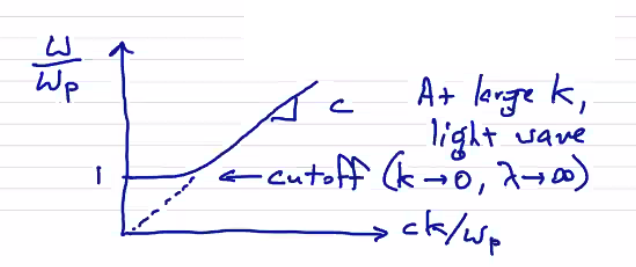
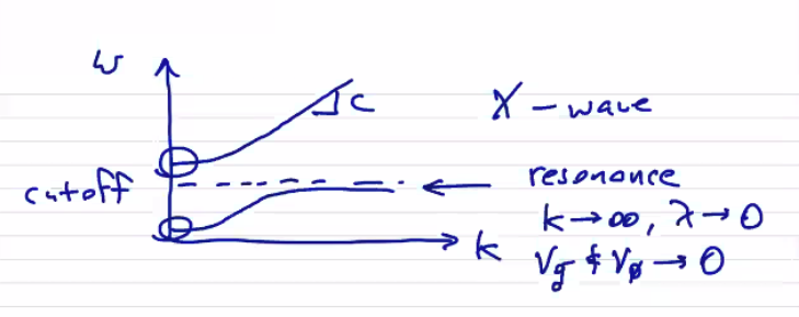
It turns out that the dispersion relation for the X-wave has the same cut-off, but also has another branch with a resonance
The two-fluid plasma model is highly reduced from the full kinetic model, but it is still too complete to be useful when studying gross plasma behavior. Further reductions of the model are possible by making asymptotic assumptions:
Low-frequency Asymptotic Assumption#
- Eliminate high frequency, short wavelength phenomena by using pre-Maxwell field equations. Formally, this is \( \epsilon_0 \rightarrow 0 \) .
The direct consequences of the low-frequency approximation are
\[c^2 = \frac{1}{\epsilon_0 \mu_0} \qquad c \rightarrow \infty\] \[\omega_p ^2 = \frac{n e^2}{\epsilon_0 m} \qquad \omega_p \rightarrow \infty\] \[\lambda_D = \frac{v_T}{\omega_p} \rightarrow 0\]
This means that all phenomena will have \( \omega \ll \omega_p \) , limiting the frequencies we can resolve to the ion plasma frequency. The characteristic speeds will be limited by the speed of light
\[\frac{\omega}{k} \ll c\]and all characteristic lengths will be much greater than the Debye length
\[x_0 \gg \lambda_D\]Looking at Gauss’ law, \[\epsilon_0 \div \vec E = \sum_\alpha q_\alpha n_\alpha \rightarrow \sum_\alpha q_\alpha n_\alpha = 0\]
so we now have charge neutrality everywhere in the domain. For H plasma, locally we have \( n_e = n_i \) everywhere.
Looking at Ampere’s law,
\[\epsilon_0 \pdv{\vec E}{t} = \frac{1}{\mu_0} \curl \vec B - \sum_\alpha q_\alpha n_\alpha \vec v_\alpha = 0 \\ \rightarrow \vec j = \frac{1}{\mu_0} \curl \vec B\]Things we do not get from this approximation are \( \vec E = 0 \) or \( \pdv{\vec E}{t} = 0 \) . It does mean that plasma dynamics occur on a sufficiently large spatial scale that charge separation is small, and they occur on a sufficiently long temporal scale that electrons respond quickly.
Tiny electron asymptotic assumption#
2nd approximation: neglect electron inertia in the momentum equation. Formally, we let the electron mass \( m_e \rightarrow 0 \)
\[\omega_{pe}^2 = \frac{n e^2}{\epsilon_0 m_e} \rightarrow \infty\] \[\omega_{c, e} = \frac{e B}{m_e} \rightarrow \infty\] \[v_{T, e} \rightarrow \infty\] The Larmor radius goes to zero \[r_{l, e} = \frac{v_{T, e}}{\omega_{c, e}} \rightarrow 0\] Importantly, as the gyroradius \( r_{l, e} \) goes to 0 (because the thermal velocity goes as \( \sqrt{m_e} \) and the cyclotron frequency goes as \( m_e \) ), this means that the electrons are tied to the magnetic field. The skin depth is also small. \[\delta_e = \frac{c}{\omega_{p, e}} \rightarrow 0\]
So all phenomena that we capture must have \( \omega \ll \omega_{p, e} \) , \( \omega \ll \omega_{c, e} \) , and \( x_0 \gg r_{L, e} \) , \( x_0 \gg \delta_e \) .
The electron momentum equation becomes
\[\grad P_e + \div \vec \Pi _e + e n_e (\vec E + \vec v \cross \vec B) = \sum_{\beta \neq \alpha} \vec R_{\alpha \beta}\]The momentum equation is now a state equation, not an evolution equation. It now simply relates the dynamical variables to each other at any point in time.
Now, note that along magnetic field lines electrons can travel long distances at very fast (finite) speeds which can produce low frequency, long wavelength phenomena. Neglecting electron inertia implies that electrons respond instantaneously, meaning we cannot capture these modes. An example of such a phenomena is drift waves.
The characteristic speeds \( c \) and \( v_{T, e} \) have disappeared from the model. Remaining is \( v_{T, i} \) . This means that the ion dynamics dictate the plasma evolution.