Magnetohydrodynamic (MHD) Model#
Applying approximations to the two-fluid plasma model will allow us to arrive at a single-fluid (center-of-mass) description. The result is the ideal magnetohydrodynamic model (MHD).
First, define the MHD variables:
\[\text{mass density:} \qquad \rho = n_i m_i + n_i m_e\] \[\text{fluid velocity:} \qquad \vec v = \frac{n_i m_i \vec v_i + n_e m_e \vec v_e}{n_i m_i + n_e m_e}\] \[\text{current density:} \qquad \vec j = q_i n_i \vec v_i - e n_e \vec v_e \rightarrow \vec v_e = \frac{q_i n_i \vec v_i}{e n_e} - \vec j / e n_e\] \[\text{total pressure:} \qquad p = p_i + p_e = n_e T_e + n_i T_i\] \[\text{total temperature:} \qquad T = \frac{n_i T_i + n_e T_e}{(n_i + n_e)/2}\]Now let’s begin applying asymptotic approximations. For the mass density, applying the first approx (charge neutrality) we have
\[\rho \approx n (m_i + m_e)\]Using approx 2 (vanishing electron mass)
\[\rho \approx n m_i\] where \[n = n_i \qquad n_e = Z n\]
The center-of-mass velocity (charge neutrality) gives
\[\vec v \approx \frac{m_i \vec v_i + m_e Z \vec v_e}{m_i + Z m_e}\]with small electron mass approximation:
\[\vec v \approx \vec v_i\]The current density is (charge neutrality approx)
\[\vec j \approx Z e n (\vec v_i - \vec v_e) \qquad \vec v_e = \vec v_i - \vec j / Z e n\]The pressure and total temperature are (with charge neutrality)
\[P \approx n (T_i + Z T_e)\] \[T \approx \frac{T_i + Z T_e}{(1 + Z)/2}\]MHD Momentum Equation#
Now we combine the two-fluid equations with these asymptotic approximations to obtain the governing equations for the MHD variables. Multiplying the ion continuity equation by the ion mass gives
\[\pdv{}{t} (m_i n_i) + \div (m_i n_i \vec v_i) = 0 \\ \rightarrow \pdv{\rho}{t} + \div (\rho \vec v) = 0 \quad \text{(MHD continuity eq.)}\]If we multiply the two-fluid continuity equations by the charge and sum them, we get
\[\pdv{}{t}(q_i n_i - e n_e) + \div (q_i n_i \vec v_i - e n_e \vec v_e) = 0 \\ \rightarrow \div \vec j = 0 \quad \text{(no accumulation of charge)}\]If we add the electron and ion momentum equations and apply the small electron mass approximation, and recognizing that \( \vec R_{ei} = - \vec R_{ie} = n e \eta \vec j \)
\[\rho_i \left(\pdv{\vec i}{t} + \vec v_i \cdot \grad \vec v_i \right) + \grad (P_i + P_e) + \div (\vec \Pi _i + \vec \Pi_e) \\ \qquad - (q_i n_i - e n_e) \vec E - (q_i n_i \vec v_i - e n_e \vec v_e) \cross \vec B = 0\] \[\text{MHD Momentum Equation} \\ \rightarrow \rho \left(\pdv{\vec v}{t} + \vec v \cdot \grad \vec v \right) + \grad p - \vec j \cross \vec B = - \div (\vec \Pi _i + \vec \Pi _e)\]
“MHD Momentum Equation”
\[\rho \left(\pdv{\vec v}{t} + \vec v \cdot \grad \vec v \right) + \grad p - \vec j \cross \vec B = - \div (\vec \Pi _i + \vec \Pi _e)\]
If we take the electron momentum equation, apply the small electron mass asymptotic approximation and introduce the current density, then we have
MHD Ohm’s Law#
\[e n_e (\vec E + \vec v_i \cross \vec B - \vec j \cross \vec B / Z e n) = - \grad P_e - \div \vec \Pi_e + \vec R_{ei}\]Substituting \( \vec R_{ei} = e n_e \eta \vec j \) \[\text{MHD Generalized Ohms Law}\\ \vec E + \vec v \cross \vec B = \eta \vec j + \frac{1}{Z e n} \left(\vec j \cross \vec B - \grad p_e - \div \vec \Pi_e \right)\]
“MHD Generalized Ohms Law”
\[\vec E + \vec v \cross \vec B = \eta \vec j + \frac{1}{Z e n} \left(\vec j \cross \vec B - \grad p_e - \div \vec \Pi_e \right)\]
MHD Energy Equation#
The energy equation is found by adding the ion and electron energies, but first we need to manipulate them into a common form. The ion energy equation is
\[\frac{1}{\gamma - 1} \left[ \pdv{}{t} (n_i T_i) + \div (n_i T_i \vec v_i) \right] + n_i T_i \div \vec v_i = RHS_i\]where \( RHS_i \equiv - \vec \Pi_i \cdot \cdot \grad \vec v_i - \div \vec h_i + Q_{ie} \)
\[\frac{1}{\gamma - 1} \left( \pdv{p_i}{t} + \vec v_i \cdot \grad p_i \right) + \frac{\gamma}{\gamma - 1} p_i (\div \vec v_i) = RHS_i\]Multiply by \( \frac{\gamma - 1}{n_i ^\gamma} \) and define the total derivative with respect to the ion velocity as
\[\dv{}{t} \equiv \pdv{}{t} + \vec v_i \cdot \grad\] \[\rightarrow \dv{}{t} \left( \frac{p_i}{n_i ^\gamma} \right) - p_i \dv{}{t} \left( \frac{1}{n_i ^\gamma} \right) + \frac{\gamma p_i}{n_i ^\gamma} \div \vec v_i = \frac{\gamma - 1}{n_i ^\gamma} RHS_i\]Simplify further by recognizing that carrying out the total derivative gives
\[\dv{}{t} \left( \frac{p_i}{n_i ^\gamma} \right) - \frac{\gamma p_i}{n_i ^{\gamma + 1}} \dv{}{t} n_i + \frac{\gamma p_i}{n_i ^\gamma} \div \vec v_i = \frac{\gamma - 1}{n_i ^\gamma} RHS_i\]The continuity equation says \[\dv{}{t} n_i = - n_i \div \vec v_i\] Multiply by \( m_i ^{- \gamma} \) and use \( \rho = n m_i \) and the resulting ion energy equation is
\[\dv{}{t} \left( \frac{p_i}{\rho ^\gamma} \right) = \frac{\gamma - 1}{\rho ^\gamma} RHS_i\]We want to get the electron energy equation in the same form. The steps are very similar:
\[\dv{}{t} \left( \frac{p_e}{n_e ^\gamma} \right) + \vec v_e \cdot \grad \left( \frac{p_e}{n_e ^\gamma} \right) = \frac{\gamma - 1}{n_e ^\gamma} RHS_e\]Since we’ve defined our center-of-mass reference frame to be that of the ions, we can not use the same total derivative
\[\pdv{}{t} + \vec v_e \cdot \grad \neq \dv{}{t}\]We now apply the charge neutrality approximation
\[n_e = Z n \qquad \vec v_e = \vec v_i - \frac{1}{Z e n} \vec j\] \[\rightarrow \dv{}{t} \left( \frac{p_e}{Z^\gamma n^\gamma} \right) + \vec v_i \cdot \grad \left( \frac{p_e}{Z^\gamma n^\gamma} \right) = \frac{1}{Z e n} \vec j \cdot \grad \frac{p_e}{Z^\gamma n^\gamma} + \frac{\gamma - 1}{Z^\gamma n^\gamma} RHS_e\]Multiply by \( (Z / m_i)^\gamma \) and the result is
\[\dv{}{t} \frac{p_e}{\rho ^\gamma} = \frac{1}{Z e n} \vec j \cdot \grad \frac{p_e}{\rho^\gamma} + \frac{\gamma - 1}{\rho^\gamma} RHS_e\]Finally we can add the ion energy equation to the electron energy equation to get
\[\dv{}{t} \left( \frac{p}{\rho^\gamma} \right) = \\ \frac{\gamma - 1}{\rho^\gamma} \left[ Q_{ie} + Q_{ei} - \div (\vec h_i + \vec h_e) - \vec \pi_i \cdot \cdot \grad \vec v_i - \vec \Pi_e \cdot \cdot \grad \vec v_e \right] + \frac{\vec j}{Z e n} \cdot \grad \frac{p_e}{\rho^\gamma}\]“MHD Energy Equation”
\[\dv{}{t} \left( \frac{p}{\rho^\gamma} \right) = \frac{\gamma - 1}{\rho^\gamma} \left[ Q_{ie} + Q_{ei} - \div (\vec h_i + \vec h_e) - \vec \pi_i \cdot \cdot \grad \vec v_i - \vec \Pi_e \cdot \cdot \grad \vec v_e \right] + \frac{\vec j}{Z e n} \cdot \grad \frac{p_e}{\rho^\gamma}\]
Obviously, we’ve retained a number of terms that are specific to the behavior of the electrons. It is possible to incorporate the electron behavior by using a single-fluid MHD model with two temperatures \( T_i \neq T_e \) . One can imagine a hierarchy of models, in which the most simplified is the single-fluid MHD model in which you evolve \( \rho \) , \( \vec v \) , and \( T \) . Moving up a level, you have a MHD model with two temperatures in which you evolve \( \rho \) , \( \vec v \) , \( T_i \) , and \( T_e \) . Upwards from there you move back into the realm of multi-fluid models.
Now to relate the fields back to source terms. The low-frequency Maxwell’s equations are
\[\pdv{\vec B}{t} = - \curl \vec E\] \[\vec j = \frac{1}{\mu_0} \curl \vec B\] \[\div \vec B = \div \vec E = 0\]
Like in the multi-fluid plasma model, we still need to close the system by expressing some of our variables using equations of state ( \( \vec h \) , \( \vec \Pi \) ).
To simplify further, we can make some assumptions about heat flow
\[\text{isothermal} \qquad \rightarrow p \propto n \qquad T = \text{const.} \qquad \gamma = 1\] \[\text{adiabatic} \qquad \rightarrow p \propto n^\gamma\] \[\text{cols plasma / force-free} \qquad \rightarrow p = \text{const.} \qquad \gamma = 0\]
Ideal MHD Model#
The extended MHD equations are simpler than the two-fluid model, but they can still be quite complicated. We can often still get useful analysis from further reductions. The ideal MHD model is such a reduction that we can get by dropping (with justification) several terms from the extended model. We justify the simplifications by comparing the magnitude of the neglected terms to the terms that are retained.
Recall the characteristic speed is \( v_{T, i} \) . If we say that the characteristic length plasma length is \( L \) , then we can define characteristic time \( \tau = L / v_{T, i} \) .
The derivation of the two-fluid plasma model assumed a Maxwellian velocity distribution. We need the velocity distribution to thermalize, reach local thermodynamic equilibrium, and become Maxwellian. This means that we need many collisions, in fact so many collisions occurring frequently enough that we can ignore collisional effects. There must then be many collisions during the characteristic time \( \tau \) .
For ions to be thermalized,
\[\frac{\tau_{ii}}{\tau} \ll 1\]And similarly for electrons
\[\frac{\tau_{e}}{\tau} \ll 1\]The continuity equation remains unchanged from the extended MHD model
“Ideal MHD Continuity Equation”
\[\pdv{\rho}{t} + \div (\rho \vec v) = 0\]
The momentum equation is
\[\rho \left( \pdv{\vec v}{t} + \vec v \cdot \grad \vec v \right) + \grad p - \vec j \cross \vec B = - \div (\vec \Pi_e + \vec \Pi_e)\] Drop the anisotropic pressure
“Ideal MHD Momentum Equation”
\[\rho \left( \pdv{\vec v}{t} + \vec v \cdot \grad \vec v \right) + \grad p - \vec j \cross \vec B = 0\]
The generalized Ohm’s law is
\[\vec E + \vec v \cross \vec B = \eta \vec j + \frac{1}{Z e n} \left( \vec j \cross B - \grad p_e - \div \vec \Pi_e \right)\]We’re going to drop the entire right hand side
“Ideal MHD Generalized Ohm’s Law”
\[\vec E + \vec v \cross \vec B = 0\]
For the energy equation we have
\[\dv{}{t} \left( \frac{p}{\rho^\gamma} \right) = \frac{\gamma - 1}{\rho^\gamma} [Q_{ie} + Q_{ei} - \div (\vec h_i + \vec h_e) - \vec \Pi_i \cdot \cdot \grad \vec v_i - \vec \Pi_e \cdot \cdot \grad \vec v_e] + \frac{\vec j}{Z e n} \cdot \grad \frac{p_e}{\rho^\gamma}\]We neglect the entire right-hand side
“Ideal MHD Energy Equation”
\[\pdv{\rho}{t} + \div (p \vec v) = (1 - \gamma) p \div \vec v \]
Collision/Pressure terms#
If we assume that the ions and electrons are in thermal equilibrium \( T_i = T_e \) , we can relate the collision times
\[\tau_{ee} : \tau_{ii} : \tau_{ei} = 1 : \left( \frac{m_i}{m_e} \right) ^{1/2} : \frac{m_i}{m_e}\]The collision times are specifically collisional relaxation times of the Boltzmann equation
\[\left. \pdv{f}{t} \right|_{coll} = \frac{f - f_{\text{Maxwellian}}}{\tau_{\alpha \beta}}\]For electrons, the thermalization condition is much stricter for the ions
\[\frac{\tau_{ee}}{\tau} = \left( \frac{m_e}{m_i} \right)^{1/2} \frac{\tau_{ii}}{\tau} \ll 1\]Neglect the anisotropic pressure tensor in the momentum and generalized Ohm’s law, \( \div \vec \Pi \) . \( \vec \Pi \) is primarily the shear stress tensor. The ion thermal speed gives us a characteristic velocity for the plasma, so we use it to characterize the shear stress
\[\vec \Pi_{i, max} \sim 2 \mu \left( \pdv{u}{x} - \frac{1}{3} \div \vec v \right) \sim \mu \frac{v_{T, i}}{L}\]Standard treatments of the viscosity (Braginskii, etc.) show that viscosity scales with the number density, temperature, and collision time
\[\mu \sim n T_i \tau_{ii} \sim p_i \tau_{ii}\] \[\Pi_{i, max} \sim p_i \frac{\tau_{ii} v_{T, i}}{L}\]The specific term we want to get rid of is \( \div \vec \Pi \) , so let’s compare it to a term we want to keep \( \grad P \)
\[\frac{\div \vec \Pi}{\grad p} \sim \frac{p_i \tau_{ii} v_{T, i} / L^2}{p_i / L} \sim \frac{\tau_{ii}}{\tau}\]So, to neglect the anisotropic pressure term in the momentum equation, once again we require
\[\frac{\tau_{ii}}{\tau} \ll 1\]In other words, as long as the plasma is collision-dominated, we can drop the ion anisotropic pressure term. What about associated the electron term? If you can assume \( T_i \approx T_e \) . Then \( p_i \approx p_e \) for a neutral plasma, and
\[\frac{\div \vec \Pi_e}{\grad p} \sim \frac{p_i \tau_{ee} v_{T, i} / L^2}{p_i / L} \sim \frac{\tau_{ee}}{\tau} \ll 1\]Magnetic terms#
In the generalized Ohm’s law, the diamagnetic drift term is
\[\frac{\grad p_e}{Z e n} \sim \frac{n T_e / L}{Z en} \sim \frac{T_i / L}{Ze} \sim \frac{m_i v_{T, i}^2}{L Z e}\]Compare \( \grad p_e / Z e n \) to a term that we’re going to keep, which is the dynamo term \( \vec v \cross \vec B \)
\[\frac{ \grad p_e / Z en}{|\vec v \cross \vec B|} \sim \frac{m_i v_{T, i}^2}{LZe}{v_{T, i} B} \sim \frac{m_i}{ZeB}\frac{v_{T, i}}{L} = \frac{v_{T, i}}{\omega_{c, i}} \frac{1}{L} \sim \frac{r_{L, i}}{L} \ll 1\]So to neglect the diamagnetic drift term, we need the plasma to be well-magnetized. This means the Larmor radius must be much less than the plasma characteristic length \( r_{L, i} \ll L \)
Now what can we do with the Hall term \( \frac{\vec j \cross \vec B}{Zen} \) . For a static plasma (or one with subsonic flows):
\[\rho (\pdv{\vec v}{t} + \vec v \cdot \grad \vec v) - \grad p - \vec j \cross \vec B = 0\]so by “subsonic” we mean that the static pressure is much larger than the dynamic pressure and we can discard the \( \vec v \) terms.
\[\vec j \cross \vec B \approx \grad p\]Comparing the Hall term to the dynamo term \( \vec v \cross \vec B \) also gives the same requirement
\[\frac{r_{L, i}}{L} \ll 1\]How well do some real plasmas hold up to the requirements of ideal MHD? Consider field nulls in a Z-pinch or an FRC, and weakly magnetized plasmas (such as those in a Hall thruster). Clearly, the magnetization requirement does not hold up at all points in space, and ideal MHD does not necessarily apply across the whole domain.
Resistivity#
We neglect resistivity and the resistive electric field \( \eta \vec j \) in the generalized Ohm’s law
\[\eta \vec j \sim \eta \frac{\grad p}{B} \sim \frac{ \eta n T}{LB}\] \[\eta = \frac{m_e \nu_{ei}}{n e^2} = \frac{m_e}{n e^2 \tau_{ei}} = \frac{m_e ^2/ m_i}{n e^2 \tau_{ee}}\] \[\rightarrow \eta \vec j \sim \frac{m_e ^2}{e^2 L B} \frac{v_{T, i} ^2}{\tau_{ee}}\]How does it compare to \( \vec v \cross \vec B \)
\[\frac{\eta \vec j}{|\vec v \cross \vec B|} \sim \left(\frac{m_e}{m_i} \right)^2 \frac{m_i}{e ^2 B^2} \frac{v_{T, i} ^2}{L^2} \frac{L}{v_{T, i} \tau_{ee}} \sim \left( \frac{m_e}{m_i}\right)^2 \frac{v_{T, i} ^2}{\omega_{c, i} ^2} \frac{1}{L^2} \sim \left( \frac{m_e}{m_i} \right) ^{3/2} \left( \frac{r_{L, i}}{L} \right) ^{2} \frac{\tau}{\tau_{ii}} \ll 1\]This now places a lower limit on \( \tau_{ii} \) ; to neglect resistivity \( \tau_{ii} \) cannot be too low
\[\left( \frac{m_e}{m_i} \right) ^{3/2} \left( \frac{r_{L, i}}{L} \right) ^{2} \ll \frac{\tau_{ii}}{\tau} \ll 1\]Heating sources#
Neglect the collisional heating sources \( Q_{ei} \) , \( Q_{ie} \) in the energy equation. We do that by assuming that they are equal and opposite, which only happens when the temperatures are equal. In other words, we are again assuming local thermodynamic equilibrium between electrons and ions.
\[1 \gg \frac{\tau_{ei}}{\tau} = \left( \frac{m_i}{m_e} \right)^{1/2} \frac{\tau_{ii}}{\tau} \rightarrow \frac{\tau_{ii}}{\tau} \ll \left( \frac{m_e}{m_i} \right) ^{1/2}\]This is a much more restrictive condition than ion collisionality. Alternatively, we could track two temperature independently.
We also neglect the heat flux terms \( \div (\vec h_i + \vec h_e) \) in the energy equation. Consider parallel (to the magnetic field) heat conduction which dominates since \( \kappa_\perp \ll \kappa_\parallel \) , so
\[\div \vec h \approx \grad_\parallel \cdot (\kappa_\parallel \grad_\parallel T)\] \[\grad_\parallel \cdot \left[ ( \kappa_{\parallel, i} + \kappa_{\parallel, e}) \grad_\parallel T \right]\] \[\kappa_{\parallel, e} \sim \frac{n T_e}{m_e} \tau_{ee} \qquad \text{ and } \qquad \kappa_{\parallel, i} \sim \frac{n T_i}{m_i} \tau_{ii}\] \[\frac{\kappa_{\parallel, e}}{\kappa_{\parallel, i}} \sim \frac{\tau_{ee}}{\tau_{ii}} \frac{m_i}{m_e} \sim \left( \frac{m_i}{m_e} \right) ^{1/2}\]Compare the thermal conductivity to the rate of pressure change \( \pdv{p}{t} \)
\[\frac{\grad_\parallel \cdot (\kappa_{\parallel, e} \grad_\parallel T)}{\pdv{p}{t}} \sim \frac{n T^2 \tau_{ee}/m_e L^2}{nT/\tau} \sim \left( \frac{m_i}{m_e} \right)^{1/2} \frac{\tau_{ii}}{\tau} \ll 1\]We’re back to the same requirement that we have ion-electron local thermodynamic equilibrium.
Anisotropic pressure terms in energy equation#
Neglect the anisotropic pressure terms in the energy equation. That is, \( \vec \Pi_i \cdot \cdot \grad \vec v_i \) and \( \vec \Pi_e \cdot \cdot \grad \vec v_e \) . Skipping ahead, the result is
\[\frac{\tau_{ii}}{\tau} \ll 1 \] \[\left( \frac{m_e}{m_i} \right)^{1/2} \frac{\tau_{ii}}{\tau} \frac{r_{L, i}}{L} \ll 1\]
Electron convection term#
Lastly, we neglect the electron convection term in the energy equation \( \frac{\vec j}{Zen} \cdot \grad \frac{P_e}{\rho^\gamma} \) . The result is
\[\frac{r_{L, i}}{L} \ll 1\]Conservation Law Form of MHD#
\[\pdv{}{t} q + \div \vec f = 0\]We can express momentum in conservation law form:
\[\pdv{}{t} (\rho \vec v) + \div \left[ \rho \vec v \vec v - \frac{ \vec B \vec B}{\mu_0} + (p + \frac{B^2}{2 \mu_0})\vec 1 \right] = 0\]The conservation law form for the magnetic field looks like
\[\pdv{ \vec B}{t} + \div \left[ \vec v \vec B - \vec B \vec v \right ] = 0\]And of course the energy equation for
\[E = \frac{1}{\gamma - 1} p + \frac{1}{2} \rho v^2 + \frac{ B^2}{2 \mu_0}\] \[\pdv{E}{t} + \div \left[ \left( E + p + \frac{B^2}{2 \mu_0} \right) - \left( \frac{ \vec B \cdot \vec v}{\mu_0} \right) \vec B \right] = 0\]Conservation law forms are particularly useful when considering equilibrium steady-state force balance. This means that in steady-state equilibrium we have
\[\div \left[ \rho \vec v \vec v - \frac{ \vec B \vec B}{\mu_0} + \left( p + \frac{B^2}{2 \mu_0} \right) \vec 1 \right] = 0\]We can use this relationship and integrate over various volumes to determine the relationship between the various force balance terms
Examples of equilibrium plasma confinement#
For a plasma in static equilibrium \( \vec v = 0 \rightarrow \vec j \cross \vec B = \grad p \)
\[ \div \vec T = 0 = \div \left( \right) \] \[\vec j \cross \vec B = \frac{1}{\mu_0} (\curl \vec B) \cross \vec B = \frac{1}{\mu_0} (\vec B \cdot \grad \vec B - \frac{1}{2} \grad B^2) \\ = \frac{1}{\mu_0} ( B^2 \vu e_B \cdot \grad \vu e_B + \frac{1}{2} \vu e_B \vu e_B \cdot \grad B^2 - \frac{\grad B^2}{2} )\]where \( \vu e_B = \vec B / B \)
\( \vu e_B \cdot \grad \vu e_B \) is the curvature of \( \vec B \) . Write it like a curvature
\[\vec K = - \vu r / R_c\]\[\vu e_B \vu e_B \cdot \grad B^2\] is gradient of \( B^2 \) that is parallel to B. Multiply by \( e_B \) gives the component of gradient along \( e_B \) . The difference between that and \( \grad B^2 / 2 \) gives you the perpendicular gradient
\[\vec j \cross \vec B = \frac{1}{\mu_0} (B^2 \vec \kappa - \frac{1}{2} \grad _\perp B^2) = \grad p = \grad_\perp p\]identify \( B^2 \vec \kappa \) is magnetic tension resulting from having a bent magnetic field line. \( \frac{1}{2} \grad_\perp B^2 \) is magnetic pressure. They have to balance the plasma pressure at equilibrium.
For example, consider a cylindrical plasma that’s in equilibrium with a helical magnetic field \[\vec B = B_\theta (r) \vu \theta + B_z (r) \vu z\]
How is plasma pressure profile determined by the different components of the magnetic field? If we want to maximize the amount of pressure we confine, what should be maximized/minimized?
\[\frac{B^2}{\mu_0} \vu \kappa = \grad _\perp ( p + \frac{B^2}{2 \mu_0} ) \]\( B_z \) is straight and has no curvature, so the only magnetic tension comes from \( B_\theta \) , so the magnetic tension from \( B_\theta \) must balance the total pressure.
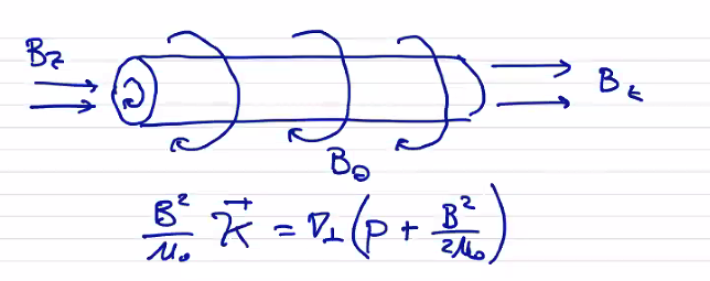
The role of \( B_z \) is displacing plasma pressure. The utility in defining \( \beta \) as
\[\beta = \frac{\text{plasma pressure}}{\text{magnetic pressure}}\]Conditions of Ideal MHD Validity#
The conditions for ideal MHD to be valid are
- High Ion Collisionality: \( \frac{\tau_{ii}}{\tau} \ll 1 \)
- Small ion Larmor radius: \( \frac{r_{L, i}}{L} \ll 1 \)
- Low resistivity: \( \left(\frac{m_e}{m_i} \right)^{3/2} \left( \frac{r_{L, i}}{L} \right)^2 \ll 1 \)
For a given plasma in force balance, we can relate the plasma pressure to the magnetic pressure
\[\beta = \frac{n T}{B^2 / 2 \mu_0} = 4 \times 10^{-16} \frac{n_{cm^{-3}} T_{keV}}{B^2 _{T}}\]Ion collision time is (Spitzer collisionality)
\[\tau_{ii} = 2.09 \times 10^{7} \frac{T_{eV} ^{3/2} \mu ^{1/2}}{\ln \Lambda n_{cm ^{-3}}} \left[\text{s}\right]\] where \( \mu \equiv m_i / m_p \) .
Putting the conditions for ideal MHD in terms of \( \beta \) and \( \tau_{ii} \) ,
- High collisionality: \[\frac{\tau_{ii}}{\tau} = 2.14 \times 10^{12} \frac{T^2}{n L} \ll 1 \] \[\rightarrow T_{eV} \ll 6.8 \times 10^{-7} L_{cm} ^{1/2} n_{cm^{-3}} ^{1/2}\]
- Small gyroradius: \[\frac{r_{L, i}}{L} = 2.3 \times 10^7 \frac{1}{Z L} \sqrt{ \frac{\mu B}{n}} \ll 1\] \[\rightarrow n_{cm^{-3}} \gg 5.3 \times 10^{14} \frac{\mu B_{T}}{Z^2 L_{cm} ^2}\]
- Low resistivity: \[\left( \frac{m_e}{m_i} \right) ^{3/2} \left( \frac{r_{L, i}}{L} \right) ^2 \frac{\tau}{\tau_{ii}} = 5.65 \frac{\mu B}{Z^2 L T^2}\] \[\rightarrow T_{eV} \gg 2.4 \frac{\mu ^{3/2} \beta^{1/2}}{Z L _{cm} ^{1.2}}\]
Perpendicular MHD#
For most configurations for magnetic fusion confinement, we are able to satisfy 2. and 3. but often have densities much too low to meet the high collisionality constraint. However, in practice ideal MHD does accurately model macroscopic behavior of many plasmas. At the same time, magnetized / fusion plasmas are often largely collisionless. We can understand why by re-writing the collisionality requirement as
\[1 \gg \frac{\tau_{ii}}{\tau} = \frac{\tau_{ii} v_{T, i}}{\tau v_{T, i}} \sim \frac{\lambda}{L}\]where \( \lambda \) is the mean free path. The ratio \( \lambda / L \) is also known as the Knudsen number. In magnetized plasmas, the mean free path is often very long, but the path between collisions can cover a great distance only by following magnetic field lines. Motion \( \perp \) to the magnetic field is constrained by \( r_{L, i} \) . This suggests an approach wherein we divide the plasma model into a 1-D kinetic model to be solved along the magnetic field and a 2-D MHD model \( \perp \) to the magnetic field.
We consider diffusivity (terms like viscosity, conductivity) parallel and perpendicular to \( \vec B \) \[k_\parallel \sim \frac{\lambda ^2}{\tau_{ii}}\] \[k_\perp \sim \frac{r_{L, i} ^2}{\tau_{ii}}\] \[\frac{k_\parallel}{k_\perp} \sim \left( \frac{\lambda}{r_{L, i}} \right)^2 \sim (\omega_{c, i} \tau_{ii} )^2\]
This changes one of our conditions for validity. Specifically, we can write
\[\frac{r_{L, i}}{L} \frac{1}{ \omega_{c, i} \tau_{i i}} = 254 \frac{\mu \beta}{Z^2 L_{cm} T_{eV} ^2}\]or
\[T_{eV} \gg 16 \frac{\mu ^{1/2} \beta^{1/2}}{Z L^{1/2}}\]This is now only slightly more restrictive than the low-resistivity condition. In fact, most of the plasmas that we looked at before (large tokamaks & toruses, propulsion systems) which had temperatures above the validity range now fall comfortably within the region of validity. The perpendicular MHD model is equivalent to a collisionless model, giving a much wider applicability than the collisional MHD model.
What about the parallel component? Our collisionality condition still isn’t valid parallel to the field. Basically, we ignore the parallel component, which is the same as assuming that \( \rho \) , \( T \) , \( p \) are constant along magnetic field lines, with \( \div \vec v = 0 \) . Let’s write out the expressions for collision-less MHD and for ideal MHD and compare:
| Collisionless MHD | Ideal MHD | |
|---|---|---|
| Continuity | \( \pdv{\rho}{t} = 0 \) | \( \pdv{\rho}{t} = - \rho \div \vec v \) |
| Momentum | \( \rho \dv{\vec v_\perp}{t} = \vec j \cross \vec B - \grad_\perp p \) | \( \rho \dv{\vec v}{t} = \vec j \cross \vec B - \grad p \) |
| Parallel constraint | \( \vec B \cdot \grad \frac{v_\parallel}{B} = - \div \vec v _\perp \) | |
| Energy | \( \dv{p}{t} = 0 \) | \( \dv{p}{t} = - \gamma p \div \vec v \) |
Collisionless MHD reproduces many of the effects of ideal MHD but has a wider region of validity. Corollary: ideal MHD is accurate beyond its region of validity, unless results lead to parallel gradients. For example, we know that MHD is not valid when representing confinement of a plasma confined in a magnetic mirror, which is an inherently kinetic phenomenon. But ideal MHD can generate parallel gradients within its region of validity, and we need to be careful. Ideal MHD does not require different models \( \parallel \) and \( \perp \) to the magnetic field, and is therefore preferred. We will continue to use ideal MHD outside of its region of validity.