Boundary Conditions #

Mathematically, a well-posed problem requires both governing equations and a complete set of boundary conditions (the Cauchy data for the problem). The most common boundary conditions we use are perfectly conducting walls (flux surfaces) or a vacuum region.

Perfectly Conducting Wall #

For the case where the plasma extends out to a perfectly conducting (impermeable) wall. Perfectly conducting walls do not support tangential electric field:

Applying Faraday’s law at the wall,

\[\left. \vu n \cdot \pdv{\vec B}{t} \right|_{wall} = \left. - \vu n \cdot \curl \vec E \right|_{wall} = \left. \div (\vu n \cross \vec E) \right| _{wall} = 0\] \[\pdv{}{t} \vu n \cdot \vec B |_{wall} = 0\] If initially there is no normal magnetic field, then \[\vu n \cdot \vec B|_{wall} = 0 \quad \text{if initially true}\]

And of course, for an impermeable wall,

Is this a sufficient set of boundary conditions? Think back to the governing equations in conservation form \[\pdv{}{t} \vec Q + \div \vec F = 0\] The boundary conditions come into play when defining \( \vec F \) at the boundary. In particular, we need to know what \( \dd \vec S \cdot \vec F |_{wall} \) is. In our governing equations, this will involve \( \vec E \) , \( \vec B \) , and \( \vec v \) .

Insulating Boundary #

As a slight modification, an insulating boundary can have a tangential electric field. Consider a simple geometry of parallel electrodes with an insulating wall between them.

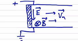
From Ohm’s law \[\vec E + \vec v \cross \vec B = 0\] so the only way an electric field tangential to the wall can exist is if \( \vu n \cdot \vec v \neq 0 \) .

For either a perfectly conducting or an insulating boundary, the other variables are arbitrary: \( \rho \) , \( p \) , \( \vec v_t \) , \( \vec B_t \) .

Vacuum Region #

The plasma (radius \( R_p \) ) is supported by a region of vacuum out to a perfectly conducting wall at some radius \( R_w \) . We assume that there is no plasma in the vacuum region. The governing equations in vacuum are just Maxwell’s equations

At the wall, \[\vu n \cross \vec E |_{wall} = 0\] \[\left. \vu n \cdot \pdv{\vec B}{t} \right|_{wall} = 0\]

What happens at the plasma-vacuum interface? We need to specify jump conditions and continuity conditions. Let’s use square brackets to signify a jump:

The normal magnetic field has to be continuous.

The tangential magnetic field jump is given by the surface current density at the jump

Integrating \( \grad_\perp (p + \frac{B^2}{2 \mu_0}) = \frac{B^2}{\mu_0} \vec \kappa \) over a differential volume across the surface gives

The plasma shape is determined self-consistently by the wall shape and surface current. This is a free-boundary problem. Another option is to specify the plasma shape, and then determine the required wall shape. This is a fixed-boundary problem.

The most realistic case includes externally applied magnetic fields coming from source coils, perhaps computed by Biot-Savart law. The vacuum magnetic field is then \( \vec B_{vac} = \vec B_{ext} + \vec B_{plasma} \) . The crazy coil shapes in the stellarator design come from the 3D geometry computations solving this problem.

Conservation of Magnetic Flux (“Frozen-In” Flux) #

Locally, \( \vec E + \vec v \cross \vec B = 0 \) with Faraday’s law \[\pdv{B}{t} = - \curl \vec E = - B \div \vec v + \vec B \cdot \grad \vec v - \vec v \cdot \grad B\] From the continuity equation, \[\pdv{\rho}{t} + \vec v \cdot \grad \rho = - \rho \div \vec v\] Combining we find that \[\dv{\vec B}{t} = \frac{\vec B}{\rho} \dv{\rho}{t} + \vec B \cdot \grad \vec v\] \[\rightarrow \dv{}{t} \left( \frac{\vec B}{\rho} \right) = \frac{\vec B}{\rho} \cdot \grad \vec v\]

This says that the field and plasma density move together. Locally, if the magnetic field increases then mass density increases, such that the ratio \( \vec B / \rho \) remains constant. In the direction parallel to the magnetic field we have a term that involves field line twisting, which is a bit more complicated, but in the perpendicular direction \[\dv{}{t} \left( \frac{\vec B}{\rho} \right) _\perp = 0\]

If we consider globally the magnetic flux through a moving surface S at velocity \( \vec u \) . The magnetic flux penetrating the surface is \[\Psi = \int \vec B \cdot \dd \vec S\] or \[\dv{\Psi}{t} = \int \dv{\vec B}{t} \cdot \vu n \dd S\] \[= \int \pdv{\vec B}{t}\cdot \vu n \dd S + \oint \vec B \cross \vec u \dd \vec l\] Using Faraday’s law

\[\dv{\Psi}{t} = \int - \curl \vec E \cdot \vu n \dd S + \oint \vec B \cross \vec u \cdot \dd \vec l\] \[= \oint (- \vec E + \vec B \cross \vec u) \cdot \dd \vec l\] Using the electric field from Ohm’s law \[\dv{\Psi}{t} = \oint(\vec v - \vec u) \cross \vec B \cdot \dd \vec l\] This tells us that if the surface moves with the plasma \( \vec u = \vec v \) then \[\dv{\Psi}{t} = 0\] the flux through the surface is constant, and the flux is a constant of the topology. This is a direct consequence of ideal MHD. If we add even a small amount of resistivity, we dramatically alter the results in a process called “tearing” where the magnetic field “tears” and reconnects with itself.