2D Equilibria#
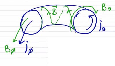
Let’s connect the ends of our 1D equilibria. Doing so is what gives us inherently toroidal configurations. From the 1-dimensional picture:
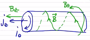
we move to an axisymmetric 2-dimensional torus, replacing our cylindrical coordinate system with a toroidal one
Eventually, the toroidal force balance will lead to the Grad-Shafranov Equation, which tells us how we can solve for a general equilibrium that solves \( \vec j \cross \vec B = \grad p \) .
Let’s consider how we might achieve such a configuration. A toroidal magnetic field can be achieved by driving current through a poloidal coil. A more complicated problem is how to drive toroidal current. In general this is done by means of a transformer, where the plasma itself is the secondary circuit. Driving a time-varying current through the primary induces a toroidal current through the plasma. This is called a transformer drive for current.
Grad-Shafranov equation#
Computing \( j_\theta \) and \( B_\phi \) can be computationally difficult in a toroidal geometry, so let’s do some work towards simplifying our force balance expression. The toroidal magnetic vector potential is defined as
\[\vec B_\theta = \curl \vec A_\phi\]If we integrate \( B_\theta \) over a poloidal surface, Stokes’ theorem gives
\[\int _{S_p} \curl \vec A_\phi \cdot \dd \vec S = \oint \vec A_\phi \cdot \dd \vec l \\ = \int _{S_p} B_\theta \cdot \dd \vec S = \Psi _p \]If the equilibrium is axisymmetric, \( A_\phi \) must be uniform along \( \dd l \) , so
\[A_\phi \vu \phi \cdot \oint \dd \vec l = A_\phi 2 \pi R = \Psi _p \\ \rightarrow A_\phi = \frac{ \Psi_p}{R} \vu \phi\]where we absorb the factor of \( 2 \pi \) into the poloidal flux \( \Psi _p \) . After some manipulation, we can relate \( B_\theta \) to the poloidal flux
\[\vec B_\theta = \curl \vec A_\phi = - \frac{ \vu R}{R} \pdv{\Psi}{z} + \frac{\vu z}{R} \pdv{\Psi}{R}\] \[\mu_0 j_\phi \cross B_\theta = (\curl \vec B_\theta) \cross \vec B_\theta \\ = \curl \vec B_\theta \cross \left( \grad \Psi \cross \frac{\vu \phi}{R} \right) \\ = - \left[ \pdv{}{R} \left( \frac{1}{R} \pdv{\Psi}{R} \right) + \frac{1}{R} \pdv{\Psi ^2}{z^2} \right] \cdot \left[\frac{ \grad \Psi}{R} ( \vu \phi \cdot \vu \phi) - \frac{ \phi}{R} \cancel{(\grad \Psi \cdot \vu \phi)} \right]\]That gives the first component of \( \grad p \) , now let’s do the other one
\[\mu_0 \vec j_\theta \cross \vec B_\phi = ( \curl \vec B_\phi) \cross \vec B_\phi \\ = \left[ - \vu R \pdv{B_\phi}{z} + \vu z \frac{1}{R} \pdv{}{R} ( R B_\phi) \right] \cross \vec B_\phi \\ = - \frac{B_\phi}{R} \left[ \vu R \pdv{}{R} (R B_\phi) + \vu z \pdv{}{z} (R B_\phi) \right] \\ = - \frac{B_\phi}{R} \grad (R B_\phi)\]Finally, since pressure is a flux surface quantity we can write
\[\grad p = \dv{p}{\Psi} \grad \Psi = p' \grad \Psi\]The toroidal force balance now looks like
\[\mu_0 p' \grad \Psi = - \frac{1}{R} \left( \pdv{}{R} \frac{1}{R} \pdv{\Psi}{R} + \frac{1}{R} \pdv{^2 \Psi}{z^2} \right) \grad \Psi - \frac{B_\phi}{R} \grad(R B_\phi)\]We notice that the only vector quantities here are \( \grad \Psi \) and \( \grad (R B_\phi) \) , so \( \grad (R B_\phi) \) must be parallel to \( \grad \Psi \) and is a flux surface quantity. We can define our new flux surface quantity as
\[F(\Phi) \equiv R B_\phi = \frac{\mu_0 I_\theta}{2 \pi} = \frac{\mu_0}{2 \pi} \int_{S_p} \vec j_\theta \cdot \dd \vec S\] \[\grad F = \dv{F}{\Psi} \grad \Psi = F' \grad \Psi\]Now each term in the toroidal force balance has a factor of \( \grad \Psi \) attached. Let’s multiply through by \( R^2 \) and factor out the gradient to arrive at the Grad-Shafranov equation:
\[R^2 \mu_0 p' = - \Delta ^\star \Psi - F F'\]where \[\Delta ^\star \equiv R \pdv{}{R} \frac{1}{R} \pdv{}{R} + \pdv{^2}{z^2}\]
To solve the Grad-Shafranov equation, you solve for \( \Psi(R, z) \) , which determines \( p(\Psi) \) and \( F(\Psi) \) , which directly gives you \( p(R, z) \) and \( F(R, z) \) and completely defines the equilibrium.
You can solve for the other terms as well. Since \( \vec B_\theta = \frac{\grad \Psi}{R} \cross \vu \phi \)
\[\vec j_\phi = - \frac{1}{\mu_0 R} \Delta ^\star \Psi \vu \phi\]and since \( \vec B_\phi = \frac{F}{R} \vu \phi \)
\[\vec j_\theta = - \frac{1}{\mu_0 R} \grad (R B_\phi) \cross \vu \phi\]For the G-S equation to be solvable, you need to specify the equilibrium by specifying \( p(\Phi) \) and \( F(\Phi) \) . In practice, this is usually done by making experimental measurements to determine \( p \) and \( F \) . A common code that does this is called EFIT, which takes the boundary conditions of the magnetic field and measurements of temperature, density to perform a least-squares fit to solve the G-S equation.
In general, the Grad-Shafranov equation leads to a matrix equation
\[\overline \vec A \vec \Psi + \vec f(\Psi) = \vec g\]Depending on the conditions we place on \( \Psi \) , \( \vec f(\Psi) \) can be a nonlinear function.
Solutions to the Grad-Shafranov equation#
In the limit that \( \vec j \parallel \vec B \) , then \( \vec j \cross \vec B = 0 = \grad p \rightarrow p' = 0 \) . These are called force-free states. In the G-S equation, the pressure term vanishes and we’re left with
\[\Delta ^\star \Psi + F F' = 0\]Spheromaks and RFPs are examples of nearly force-free states in which the current is nearly parallel to the magnetic field. Notice that in completely force-free states, \( \langle \beta \rangle = 0 \) .
Another interesting limit is the case where \( F F' \gg \Delta ^\star \Psi \) . Now we have \[\grad p \approx \vec j_\theta \cross \vec B_\phi\] which looks like a \( \theta \) -pinch which has been connected at the ends. Remember from the previous section that we can not maintain radial force balance with purely toroidal fields, so the toroidal current is not zero (hence the \( \approx \) ) but is just high enough to maintain radial force balance. This sort of configuration is called a high- \( \beta \) tokamak.
The other limit is \( F F' \ll \Delta ^\star \Psi \) \[\grad p \approx \vec j_\phi \cross \vec B_\theta\] which looks like an end-connected z-pinch. This configuration is usually called an Ohmically heated Tokamak, and the majority of currently operating tokamaks operate this way. As we know, a purely poloidal field has very bad stability properties, so \( \vec B_\phi \) needs to be added to provide stability. The toroidal \( \beta \) is very small \[\beta _t \ll 1 \qquad \beta _p \approx 1\]
Stability Considerations#
The same stability factors exist in 2D equilibria that we found for 1D equilibria:
Magnetic shear - the safety factor \( q(\Psi) = \frac{\Delta \phi}{\Delta \theta} \) for \( \Delta \theta = 2 \pi \) . We can calculate \( q \) more easily by integrating along a flux surface in the poloidal plane:
\[q(\Psi) = \frac{1}{2 \pi} \int_0 ^{\Delta \phi} \dd \phi \\ = \frac{1}{2 \pi} \int _0 ^{2 \pi} \dv{\phi}{\theta} \dd \theta \\ = \frac{1}{2 \pi} \int_0 ^{2 \pi} \dd \theta \left. \frac{r B_\phi}{R B_\theta} \right|_{\text{along flux surf.}} \\ = \frac{F(\Psi)}{2 \pi} \oint \frac{ \dd l_p}{R^2 B_\theta} \qquad \dd l_p = r \dd \theta\]Magnetic well: similarly we can get the magnetic well factor by integrating around a flux surface in the poloidal plane
\[\langle Q \rangle = \frac{\oint \frac{Q \dd l_p}{B_\theta}}{\oint \frac{ \dd l_p}{B_\theta}}\]Shafranov Shift#
Remember that when we had an equilibrium which had a toroidal current and a corresponding poloidal magnetic field, and a poloidal magnetic field, then radial force balance will tend to shift the configuration outwards away from the major axis and a conducting wall or external coil will be required to maintain the equilibrium. The radial force balance is really achieved by \( \vec j_\phi \cross B_p \)
As we move towards the magnetic axis, \( B_p \rightarrow 0 \) by definition. With less poloidal field to balance the radial force imbalance, there is more radial expansion. This means that inner portion of the plasma (inner flux surfaces) must shift radially further to achieve radial force balance.
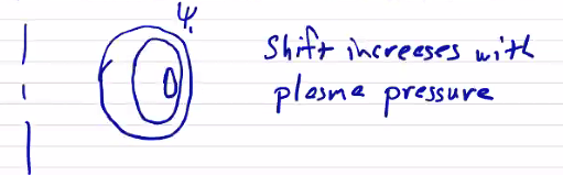
The shift increases with plasma pressure. This effect is further enhanced if we have low poloidal fields, for example in the high- \( \beta \) tokamak configurations.
Low aspect ratios also enhance the effect. Recall that the radial force imbalance increases with smaller aspect ratio, leading to a larger shift.