B-dot Probe Diagnostics #

Faraday’s law is the basis for magnetic field coils:

\[\int \pdv{\vec B}{t} \cdot \dd \vec S = - \oint \vec E \cdot \dd \vec l = - V_{emf}\]

For a rigid, perfectly conducting loop of N turns in the presence of a changing magnetic field,

\[V_i = \oint \vec E \cdot \dd \vec l = - \pdv{\Phi}{t} = - \pdv{}{t} \int \vec B \cdot \dd \vec s = - N A \frac{\int \pdv{\vec B}{t} \cdot \dd \vec s}{\int \dd \vec s} \\ \rightarrow V_i \propto \dot{B_{avg}}\]

where \( B_{avg} \) is the area-averaged magnetic field aligned to loop. The signal \( V_i \) increases with loop area, but the spatial resolution decreases. Multiple turns of coil increase the signal (effective loop area). The signal must be integrated in time to obtain the local magnetic field strength.

\[B_{avg}(t) = - \frac{1}{NA} \int_0 ^t V_i \dd t'\]

Typical probes are small for spatial resolution, and feature windings in 3 orthogonal directions. Mount the probes on insulating material to avoid perturbing local magnetic field.

B-dot Probe Calibration #

Before using a B-dot probe for diagnostics, a calibration must be performed, which involves applying a known time-varying magnetic field and recording the probe response. Consider the following experimental setup for the calibration of a B-dot probe:

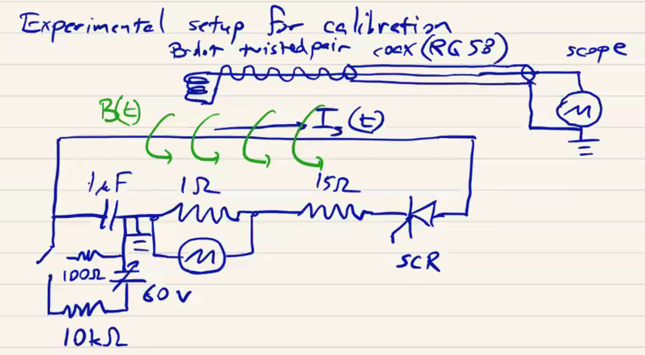
Our coil is mounted in place and connected via RG 58 to an oscilloscope. Nearby the probe, the magnetic field source is a current-carrying wire connected to a switched charging/discharge circuit as shown. When we perform the experiment, we are able to see a very clean source \( I_s(t) \)

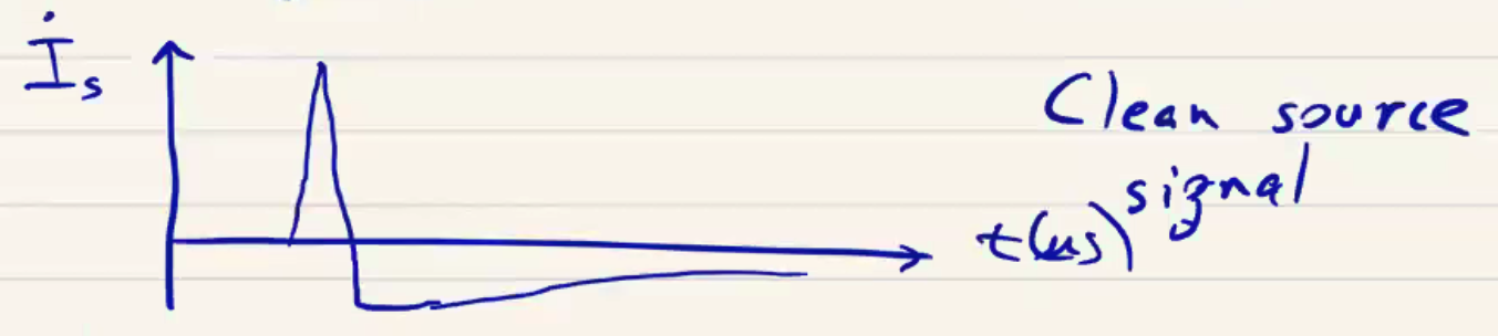
but we measure a very noisy \( V_0 (t) \) at the oscilloscope.

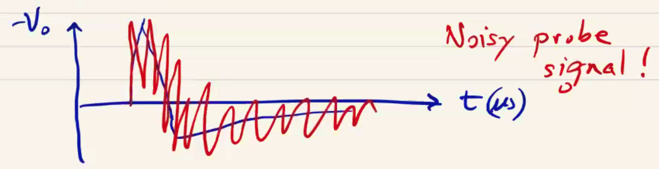
The problem is that the finite impedance of the various components of our diagnostic circuit (containing the probe itself) gives rise to resonance. We can see this by analyzing the equivalent impedance circuit. In this calibration, the following components were used:

\[L_C = 374 \mu H \\ R_C = 3.2 \Omega \\ C_C = 2 pF \\ C_{tp} = 12 oF \\ L_{coax} = 0.2 \mu H \\ C_{coax} = 70 pF \\ C_O = 20 pF \\ R_i = 1 M \Omega\]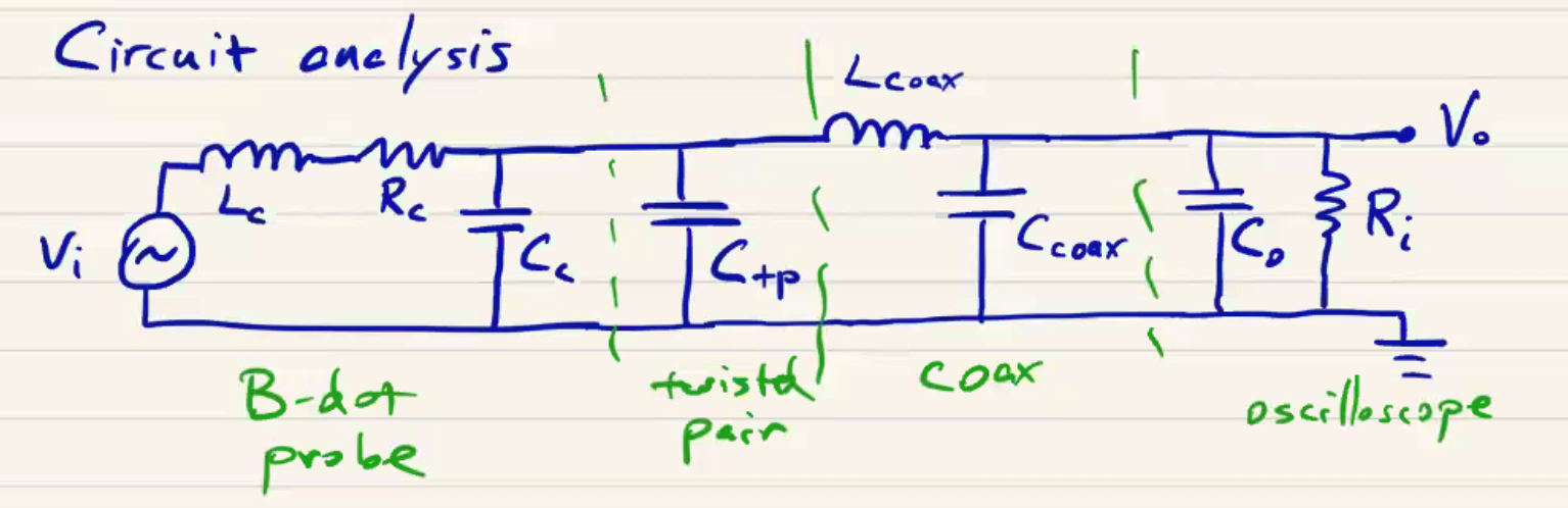

With these values, the simplified LRC equivalent circuit is:

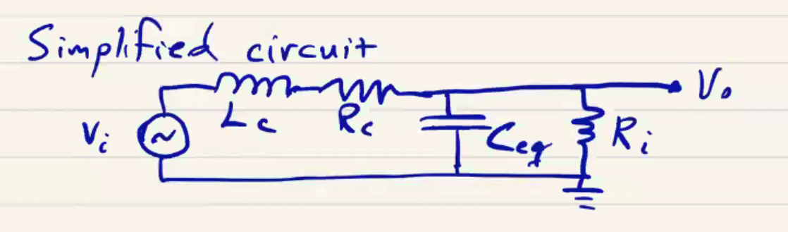
We analyze the circuit response by the method of Laplace transforms:

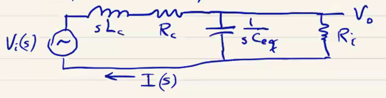
The equivalent circuit impedance to the generator voltage is then

\[Z(s) = s L_C + R_C + \frac{R_i}{1 + s C_{eq} R_i}\]

which gives a current \( I(s) = V_i(s) / Z(s) \). The output voltage is then (with some algebraic manipulation)

\[V_O (s) = \omega_0 ^2 V_i (s) \left[ s^2 + s \left( \frac{R_C}{L_C} + \frac{1}{C_{eq} R_i} \right) + \omega_0 ^2 \left( \frac{R_C}{R_i} + 1 \right) \right]^{-1} \\ \omega_0 ^2 = (L_C C_{eq} )^{-1}\]

where \( \omega_0 ^2 = (L_C C_{eq})^{-1} \). If we assume a unit step waveform for the generator voltage (that is, \( \dot B \)), then \( V_i(s) = \frac{1}{s} \) and

\[V_O(s) = \frac{\omega_0 ^2}{s (s^2 + s \alpha + \omega_0 ^2 \beta)}\]

where \( \alpha \) and \( \beta \) are the coefficients above. Taking the inverse Laplace transform (after some algebra), we arrive at

\[V_O(t) = \frac{1}{\beta} \left[ 1 - e^{- \alpha t / 2} \left( \cosh (m t) + \frac{\alpha}{2m } \sinh (m t) \right) \right]\]

where \[m^2 = \frac{\alpha^2}{4} - \omega_0 ^2 \beta\]

There are thus three possible situations:

Critically damped: \( m^2 = 0 \)
Under-damped: \( m^2 < 0 \)
Over-damped: \( m^2 > 0 \)

If we plug in the values for our experimental setup, we find \( m^2 < 0 \) and \( \frac{m}{2 \pi i} = 818 kHz \). This is the frequency of the noisy oscillations we picked up on our scope. To reduce the noise, we would like to achieve \( m^2 = 0 \), which corresponds with an input impedance of \( 950 \Omega \). Typically oscilloscopes have a high-impedance setting of \( \sim 1 M\Omega \) and a low-impedance setting of \( \sim 50\Omega \). We can leave the scope at the high-impedance setting and add a shunt resistor in parallel with the oscilloscope to adjust the input impedance to our liking.

For a realistic signal, the rise time will be finite (not a perfect step function). To track a more realistic impulse and reduce noise further, we can analyze the circuit assuming an input voltage profile that better matches the expected rise time. By doing so and carefully choosing the impedance to minimize oscillations, the voltage reported by our diagnostic circuit better represents the source, which is the magnetic field we are trying to measure!. In general, you want to set the input impedance as high as possible without generating oscillations.

If we go back to our setup and measure the probe response with different input impedances \( R_i \), we see the following:

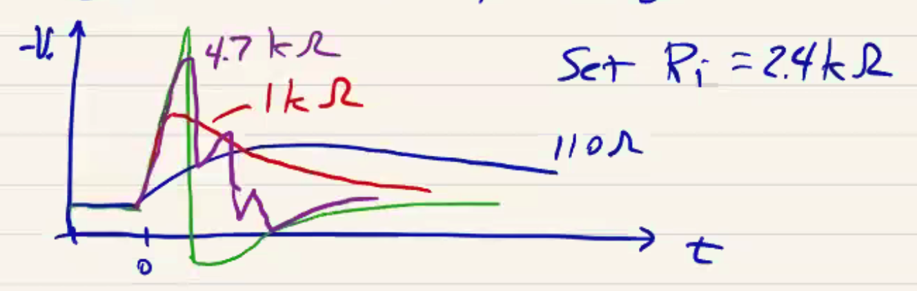
An low input impedance results in overd-amping and a smeared-out signal. At \( R_i = 4.7 k\Omega \) we see several oscillations. At \( R_i = 2.4 k\Omega \) we see a signal that closely resembles the \( \dot B \) we expect.

A similar decrease in oscillations can also be achieved using a series resistance, but this approach is susceptible to noise. Using a lower impedance is generally the preferred approach, but not always! We will see in our analysis of Rogowski coils later that impedance matching in series can be useful.

Finally, to recover the field strength \( B \) we are trying to measure, we need to integrate our signal. This can be achieved numerically from the digitization recorded by our scope. However, a digitizer is only able to record a finite bit depth, often as little as 8-bits, and a lack of precise sampling will result in drift and imprecise measurement. Typically, it is better to electronically integrate the signal by adding a passive integrator:

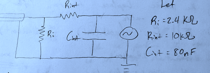
Note: the passive integrator here is a low-pass filter. After adding the integrator, we must repeat the circuit analysis with a realistic magnetic field, e.g. a triangular wave (such that \( \dot B \) becomes a square wave):

\[\mathscr{L}(\text{square}(t/a)) = \frac{\tanh(as/2)}{s}\]

and a triangular wave is defined as

\[\text{trw}(t) = \int _0 ^t \text{square}(t') \dd t'\]

Further B-dot probe considerations #

Small coils better localize the measurement. Since you’re averaging the magnetic field over the cross-sectional area of the probe, you can better localize the field. Small coils also limit the perturbation of the plasma. However, the downside is that they are more difficult to make. They are typically wound by hand (by some poor graduate student) and can be very tedious to construct (especially 3D coils with many turns). Small coils also produce smaller signals, so they require additional windings to make up for the signal loss.
Some labs have used surface-mounted inductors to make miniature B-dot probes. Surface-mounted components have many advantages in size and inductance values, and can be used as very small pickup coils for magnetic field measurements.
Additional windings increase the inductance, and this can affect the frequency response of the coil. You can always make up for the frequency response by adjusting the input impedance, but often this will decrease the signal amplitude and may cause the signal-to-noise ratio to decrease.
Active integrators can improve the bandwidth response of the probe and automatically eliminate droop and drift.

Rogowski Coils #

Rogowski coils are also fundamentally magnetic field probes, but instead of measuring the local magnetic field averaged over the coil area as B-dot probes, Rogowski coils measure the line integral of the magnetic field, which is related by Ampere’s law to the enclosed current.

If we have some plasma current \( j_z \) producing a magnetic field \( B_\theta \), then a Rogowski coil is a solenoidal coil that goes around the plasma as shown to produce a voltage \( V_0 \).

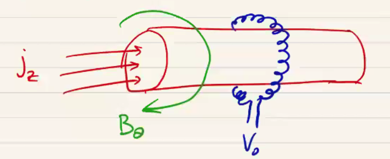
The key geometric property of the Rogowski coil is the constant inner coil radius (area).

The total magnetic flux, \( \oint \vec B \cdot \dd \vec s \), linked by the Rogowski coil is

\[\Phi = N \int \dd S \oint \vec B \cdot \dd \vec l = \mu_0 (N \int \dd S) I\]

From Faraday’s law,

\[V_0 = - \dot \Phi = \mu_0 (N \int \dd S) \dot I\]

So the voltage we measure is related to the time rate of change of the current enclosed in the Rogowski coil. The signal \( V_0 \) is integrated in time to give the total current enclosed by the Rogowski coil, \( I(t) \). Just like the B-dot probes, instead of computing the geometry of the coil we calibrate the probe by driving current from a known source and measuring the response. They are easier to calibrate because the exact geometry does not matter, as long as the Rogowski coil encloses the current being measured.

Considerations #

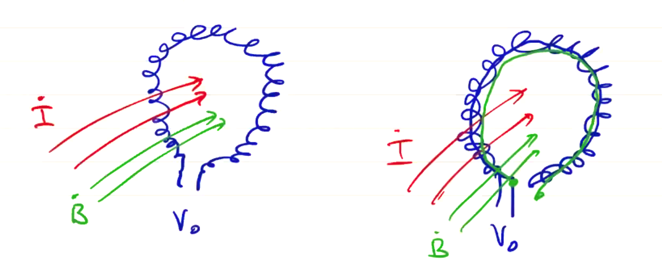
The signal is insensitive to the shape of the coil since \( \oint \vec B \cdot \dd \vec l \) is path independent. We do start to lose signal if we make the loop much larger than the source where the current source is, but as long as the coil is more or less snug about the current source the measurement error is minimal. However, the coil does need to form a complete loop.
Signals can be very large, easily \( \sim 1 kV \). So adding an attenuator upstream of your measurement circuit is important.
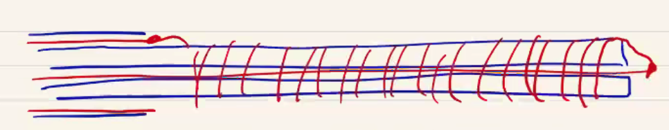
The signal can be contaminated by unwanted \( \dot{\vec B} \), so the coils are counter-wound.

In the lab, we'll often fabricate these coils by stripping the outer sheath and outer conductor from a length of RG58 coaxial cable. Then, we take a wire and solder it to the end of the inner conductor, then wrap the wire about the insulator of the RG58 back towards the un-stripped end. Finally, connect the wire to the outer conductor of the coaxial cable.

Hall Probe #

B-dot probes are not very useful for steady-state magnetic fields (it’s right there in the name). For steady-state fields, we can exploit the Hall effect. Passing a known current through a conductor with an embedded magnetic field will generate a transverse potential:

\[\frac{ \vec j \cross \vec B}{nq} = - \vec E\]

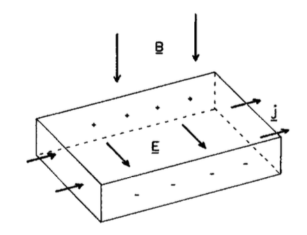
A simultaneous measurement of the voltage drop and current gives a measurement of the embedded magnetic field. Such a device is usually called a Gaussmeter.