Langmuir Probes #

Langmuir probes are the oldest and simplest plasma diagnostic: You simply insert an electrode into the plasma and measure the \( I \)-\( V \) curve. Doing so is fairly simple, but the probe measurements are often difficult to interpret, since extracting accurate plasma properties from measurements can be challenging.

Consider a probe inserted into a steady-state plasma. We assume that there is an electrode (e.g. the wall of the vacuum chamber) which is essentially in electrical contact with the plasma, and we will treat that as ground.

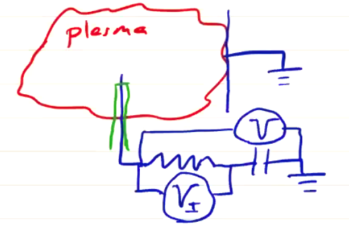
Assuming a thermal plasma (Maxwellian) with \( T_i \approx T_e \), ions and electrons strike the probe in all directions. Assume the bulk plasma is static (the bulk velocity is zero). Then the particle flux for each species \( s \) is

where \( \overline{v}_s \) is the mean particle speed. A probe of area \( A \) initially at zero potential inserted in a singly charged, quasi-neutral plasma will emit a current

A positive current here means the probe absorbs electrons. The probe potential, which started at ground, drops and repels incoming electrons until \( \Gamma _e = \Gamma _i \) such that \( I = 0 \). When this happens, we can measure the probe voltage to give what we call the “floating potential” \( V_f \). If the probe potential can be externally controlled, then we can find the floating potential without depleting the plasma of electrons. We can start out with a negative probe \( V \) and adjust it until the probe current vanishes.

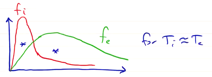
A thermal plasma by definition has a probability distribution of speed of the form

Since the electron mass is small, the speed distribution is higher than that of the ions for \( T_i \approx T_e \):

As the probe potential is more positive, eventually no electrons are repelled. This potential is the plasma potential (or space potential) \( V_p \). Increasing \( V > V_p \) further produces no increase in current, because at \( V_p \) the probe is already absorbing all of the incoming electrons.

As a point of reference, the plasma potential is approximately 5 times the electron temperature

An idealized I-V characteristic looks like this:

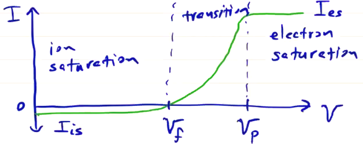
Since \( m_i \gg m_e \), \( I_{is} \ll I_{es} \). If \( T_i = T_e \) then

The transition region is where we make most of our measurements of plasma parameters. As \( V \) is adjusted between \( (V_f, V_p) \), the electron current varies exponentially as

where \[I_{es} = \frac{1}{4} e A n_e \overline{v}_e = e n_e A \left( \frac{k T_e}{2 \pi m_e} \right)^{1/2}\]

If we measure the electron current \( I_e \) vs. \( V \), this allows us a measurement to get the electron temperature \( T_e \). Note that \( I_e \) is not the total current; we need to subtract the ion current \( I_e = I - I_i \). So to recover the electron temperature, we plot \( \ln (I) \) vs. \( V \) and check the slope in the transition region:

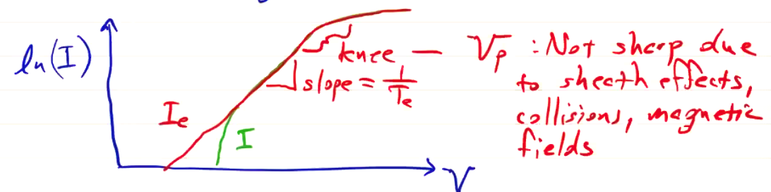
Since \( I_{is} \) is fairly constant at low \( V \), it is often easier to adjust \( I_i \) until the linear portion is maximized. With \( T_e \) determined, the density could be extracted from the electron saturation current \( I_{es} \). Looking at the form of \( I_{es} \), you can see that it depends only on the probe geometry, electron temperature, and density. So we could measure the density as

but besides being difficult to measure, \( I_{es} \) can be very large, leading to Bad Things like altering the plasma properties, damaging the probe, or destroying the probe circuitry.

Instead, we take a look at the other end of the \( I \)-\( V \) curve and determine the ion density \( n_i \) from the ion saturation current, which is generally less than \( 10 \% \) of the electron saturation current.

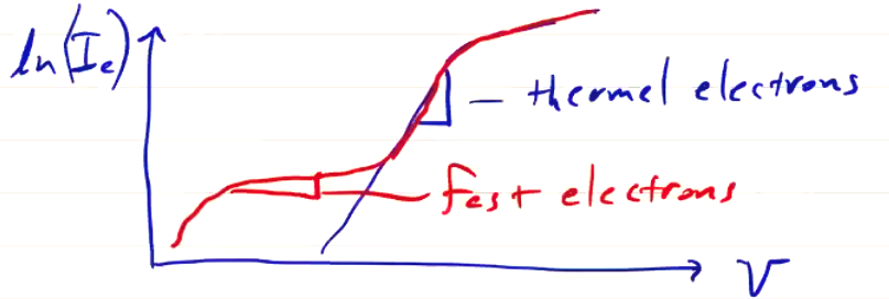
If the electrons have an energetic population (e.g. a beam or other population of high-temperature electrons) in addition to the thermal population, then the distribution is not Maxwellian. Useful information can still be obtained from the \( I \)-\( V \) characteristic, but it will contain additional inflection points

Floating Potential Measurement #

As the probe becomes more positive, it attracts more electrons, and since the probe is of finite size it reaches a point where it can’t absorb any more electrons. As the voltage increases, a sheath forms around the probe, and increases the effective area of the probe.

If we use the Bohm sheath criterion which determines a balance between the sheath thickness and ion velocities entering. Ions will be accelerated to the sound speed as they enter the sheath, and any ions less than the sound speed will be repelled away.

where \( A \) is the area of the probe, \( c_{s, i} \) the ion sound speed, and \( \alpha \) a parameter to account for the probe geometry. It is \( 1/2 \) for a planar probe, and generally falls in the range \( (0.5, 3.0) \). The ion sound speed is given by

Note that it is the electron temperature which determines the sound speed. So if \( T_e \) is known, the density can be computed from \( I_{i, s} \). To compute the floating potential, we equate the currents for charge neutrality

where \( V_f \) is the floating potential and \( V_p \) the plasma potential. Solving gives

Plasma Potential Measurement #

Ideally, we would get \( V_p \) from the point where the I-V curve departs from the linear segment. But in practice, the I-V curve is not as clean as shown and doing so can’t be done by inspection

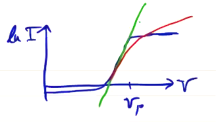
Instead, we can plot a curve of \( \dv{I}{V} \) vs \( V \) and choose the peak:

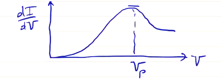
Note that whenever you differentiate experimental data, you won’t get very smooth results, especially at low \( I \) where the signal-to-noise ratio can be quite low. This is not a problem at large \( I \) where we find \( V_p \), so you can generally get a good measurement by this method.

Double and Triple Langmuir Probes #

\( V_p \) can fluctuate significantly in time, which complicates the shape of the signal and can push into the electron saturation region (and kill our probe). We can solve this problem by using a double probe, such that the entire probe floats:

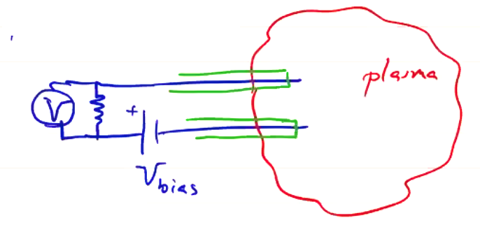
Since the entire probe floats as the plasma potential, the current is based on the bias potential and not the plasma potential with respect to ground.

In the lab we usually make Langmuir probes by taking a small piece of tungsten wire (1/16" diameter, 1" long) and insert into the tip of a hypodermic needle and solder in place. Insert the whole thing into a boron nitride cylinder. As the probe tip wears down with use, we can expose additional tungsten wire from the needle.

The way we trace I-V with a single or double Langmuir probe is by sweeping the bias potential, so that the probe potential sweeps, and measure the current. We assume that the plasma properties are quasi-constant over a period of the sweep voltage, and this assumption can limit the time resolution or applicability of the measurement. If plasma parameters are changing rapidly, instead of sweeping the voltage we can use a triple probe to measure multiple points on the I-V characteristic simultaneously.

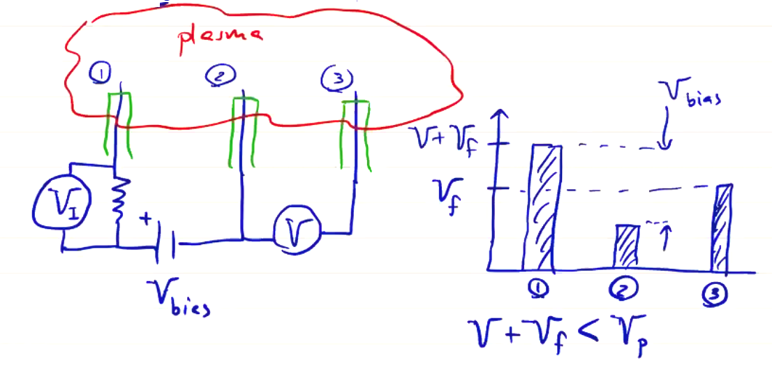
If probe 3 floats to \( V_f \), then probe 2 will be at a lower potential and probe 1 will be at a higher potential. Probe 1 will be at the measured \( V \) plus the floating potential, and the difference between probes 1 and 2 is the bias potential. Always operate such a probe such that \( V + V_f < V_p \) to avoid saturation. If \( V_{bias} \) is sufficiently large, the current through the double probe (probes 1 and 2) will be \( I_{i, s} \). The simultaneous measurement of the slope of the I-V curve gives \( T_e \) and \( I_{i, s} \) gives \( n_i \). To accomplish this, we solve for the current through each probe:

Solving these simultaneously gives

which we can solve for \( T_e \) given \( V_{bias} \) and \( V \). Another solution gives \( n_i \).

Some useful references on Langmuir probes are Chen, JAP (1965) and Qayyum, RSI (2013).

Considerations and Assumptions #

• Electrostatic probes are affected by sheath conditions and by plasma parameters. Errors can be large, \( \sim 40 \% \) for \( T_e \) and \( \sim 300 \% \) for \( n_i \)
• Probes can not be used in high-temperature or high-density plasmas (\( T_e > 20 keV\) or \( n_e > 10^{13} cm^{-3} \)). In this regime, probe effects modify the behavior and give less reliable data.
• Assume that the probe radius is much smaller than the plasma mean free path (which is to say, assume the plasma is collisionless)
• Assume that the sheath is collisionless: the Debye length is much less than the probe radius. This is what allows for the application of the Bohm criterion
• For double/triple probes, assume all probes have the same collection area and geometry
• Assume that probes are insulated to prevent arcing. High voltage difference between probe tips can cause arcing, which destroys the probe and ruins data collection.

It is possible to use probes in magnetized plasmas, sort of. Corrections exist that account for finite Larmor radius (FLR) effects, but the analysis is complicated and quite limited. Generally, we say that electrostatic probes are only valid in weakly magnetic plasmas, where the electron gyroradius \( r_{L, e} \) is much greater than the probe size.

The plasma flow velocity can be measured by adding an additional probe, forming a quadruple Langmuir probe (also called Mach probe). The probe faces the incoming plasma, and we modify the insulator to create a barrier around three of the probes. The leading probe is the Mach probe, and the shadowed portion is a triple-probe to make \( T_e \) and \( n_e \) measurements as we just described.

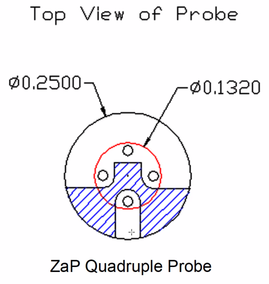
In the diagram, we see the probe tips head-on and the shaded portion is a raised insulator. The plasma flow enters from the bottom side. The Mach probe measures a current \( I_{i, s} \) that is enhanced by the plasma flow velocity \( u_{\infty} \)

Some good references for Mach probes are Hutchinson, Physics of Plasmas (1987) and Peterson, RSI (1994). There is still active debate about how best to interpret measurements. Langmuir probes are among the most simple diagnostic measurements, but assumptions and analyses are much more complicated.

Gridded Energy Analyzer (GDA) #

Also known as Retarding Potential Analyzer (RPA). Langmuir probes assume features of the distribution function and extract plasma parameters from that. In contrast, the GEA measures the distribution function \( f(v) \) more or less directly. They are typically used to measure the ion distribution function \( f_i(v) \), more specifically the energy distribution function \( f_i(\phi) = f_i (\frac{1}{2} m_i v^2) \).

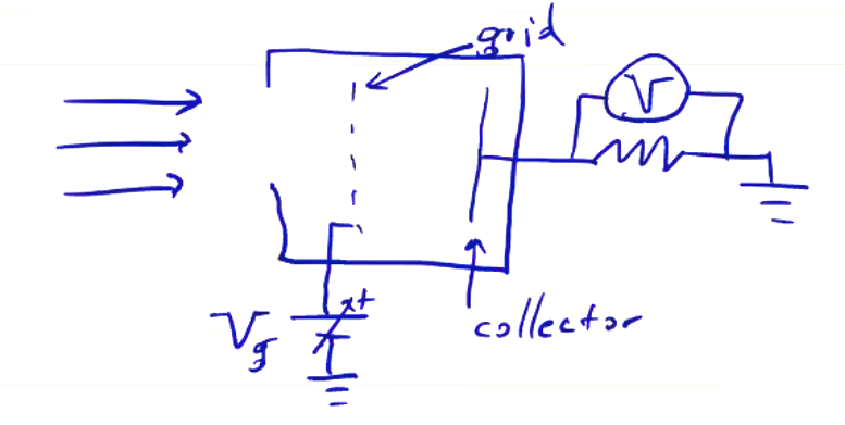
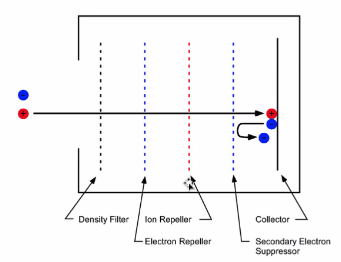
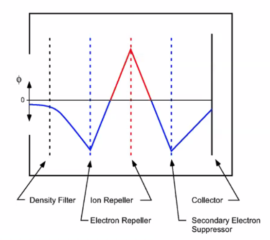
The grid voltage \( V_g \) is at a positive potential, so it is an ion repeller (also called the discriminator or gate). The way the GEA works is that only ions with an energy above \( V_g \) reach the collector. Any with energy less than \( V_g \) are repelled. The collector current (for collector area \( A_c \) is

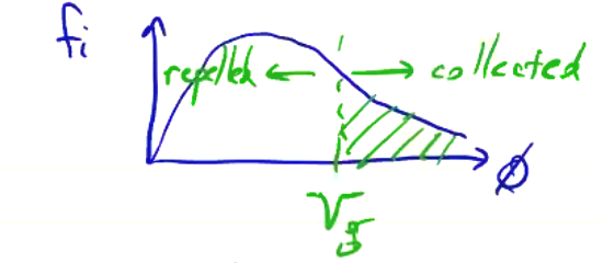
If we think back to the distribution function for ions, anything to the right of the gate voltage is collected and everything to the left is repelled, so we are collecting the high-energy tail above \( V_g \). As a function of \I( V_g \), we get the ion cumulative distribution function, and if \( f_i(\phi) \) is Maxwellian, then \( I(V_g) \) is an error function.

In a real setup, we want to collect the ions at a specific bias voltage. First, we place a density filter to decrease the plasma density. This is necessary because the Debye length needs to be large compared to the grid spacing or the grid potential will be shielded. We need to repel the electrons, so a negatively charged grid is placed to repel them. The ions are gated at a high-voltage ion repeller, then collected at the collector. When ions strike the collector, there is a chance to liberate electrons which would increase the measured current. We place a secondary electron deflector to prevent this.

Considerations for GEA/RPA #

• We need very low densities for GEA analysis. Debye shielding must not filter the grid potential, so the grid spacing must be less than the Debye length. This usually means a density filter is applied upstream.
• All electrons must be removed: this is the electron repeller grid.
• Ions will strike the collector and liberate electrons from the surface, artificially increasing the measured current (secondary electrons). As far as our ammeter is concerned, electron leaving the collector has the same effect as an ion reaching the collector.