Particle Diagnostics: Neutron diagnostics (Aria Johansen) #

Start from the basics: what is a neutron? It’s a spin \( 1/2 \) baryon which interacts with all forces. Primarily decays into usually an electron and an antielectron neutron as well as a proton. Another decay process with 1/1000 of intensity decays to gamma. Mass is \( 939.6 MeV/c^2 \), very comparable to proton.

Where do neutrons come from? They decay quite rapidly - 15 minute lifetime. #

• One of the ways you can make a neutron is through inverse beta decay - a rare process in which an electron antineutrino collides with a proton creating a neutron and positron
• Spallation from atmospheric muons - creates a background of neutrinos
• Neutron emission - larger unstable nuclei can produce free daughter neutrons (spontaneous fission, induced fission, photoneutron, spontaneous neutron emission, beta-delayed neutron emission)
• Nuclear fusion - depending on the size of the nuclei fused, neutrons of a specific energy are emitted. This is the focus of this talk and the focus of neutron diagnostics in fusion plasmas.

In a fusion reaction, neutrons come from the parent nuclei, although not every fusion reaction creates a free daughter neutron. D+T fusion in particular produces a 14.1 MeV daughter neutron and neutral \( 4He \). D+D produces a daughter neutron of 2.45 MeV and 3He about 50% of the time.

Neutron spectroscopy #

You can count the neutrons that come from a fusion reaction, and you can also look at their spectra. One of the best ways to look at the energy of the neutrons is to measure the response in a scintillator which releases a proportional number of photons

Neutron energy classification #

The general strategy for detecting neutrons is to collide them with a target nucleus, to produce a charged particle or electromagnetic interaction that can be detected. These processes are

• recoil nucleus: scintillating materials for fast neutron spectroscopy
• proton: proportional counters with high pressure He fill gas
• alpha particle: 6Li and B
• Fission fragments: 233U, 235U, 239P are the target nuclei
• Neutron energy dictates a specific detector’s desirability

Two major categories of techniques for measuring fast neutrons:

• fast neutron spectroscopy
• cool fast neutrons through mediation before counting

Neutrons of different energies are detected in different ways. Fast neutrons are our main concern (1-20MeV), as they are the products of nuclear reactions.

In the scintillator, an incident neutron causes an emission of photons from the scintillating material, which make their way to the photocathode. The photocathode feeds into the photomultiplier which feeds a substantial electric pulse. Measurement is done in a time window. The scintillator material might have a characteristic time of some tens of nanoseconds. A few common types used for fast neutron counting and spectroscopy are

• Liquid organic scintillators
• Plastic scintillators
• 3He scintillators

Liquid organics #

• Pros
  • Can distinguish neutrons from x-rays by pulse shape
  • Robust to radiation
  • Cost effective for really big detectors
• Cons
  • Slower response time (100s of ns) makes high count rate applications unreliable
  • Liquid needs a container
  • Oxygen impurity removal

3He Scintillator #

• Pros
  • Several nanosecond decay time
  • Robust to radiation
• Cons
  • Rare element using 3He
  • Hard to contain as it outgasses readily
  • Under pressure (up to 150 atm)
  • Liquid Ni cold
  • Poor pulse height resolution
  • Cross section for faster neutrons becomes small with increasing energy

Plastic Scintillator #

• Pros
  • Fast pulse response
  • Maintains its own shape
  • Easy to assemble
  • Great cross section with neutrons because of high hydrogen content and fast neutron energy range considerations
  • Decay time is generally 1-4 ns
• Cons
  • No pulse shape discrimination
  • Degrades from radiation exposure

Photodetectors used for neutron detection #

Scintillating materials make a range of photon wavelengths and numbers specific to the material and incident radiation known as a Compton spectrum

Pairing scintillators with photomultipliers requires that they have matching geometry, similar maximum emission (scintillator) and peak (PM) wavelengths

Photomultipliers have different time responses dictating their pulse resolution in time, and thus reliability with high neutron incidence. Increasing distance from source reduces incidence, increasing reliability, however more detectors need to be used for reliable counting measures.

Photomultiplier Tubes #

• Pros
  • Large range of types and characteristics available
  • Slightly higher gain and robustness to temp than a SiPM
  • Generally cheaper than SiPM
• Cons
  • Fragile and light sensitive, even when not in operation
  • Requires stable high voltage supply
  • Active area per dead time is generally greater than SiPMs
  • Some types require magnetic shielding
  • Can have smaller active area, but even with this has larger profile than SiPM

Useful PMT Terminology:

• Dynodes: produce a measurable current at anode of the photomultiplier. Usually a conductor with insulated coating.
• Gain: Total amplification of electron across PM, \( G = \delta ^n \)
• Secondary emission factor: gain of each electrode \( \delta = K V_d \)
• Linearity: when each stage in PM is proportional to initial cathode current
• Dead time (Pulse width): the finite time required by the detector to process an event
  • Extendable (paralyzable) - detector becomes insensitive to events
  • Non-extendable (non-paralyzable) - detector is still sensitive to events
• Pulse pile up: Non-extendable dead time is a distortion of signal caused by two events with overlapping dead time

Silicon Photomultipliers (SiPMs) #

• Pros
  • Small active area
  • Insensitive to magnetic fields
  • Good photo detection efficiency
• Cons
  • False positives (afterpulse/crosstalk)
  • Finite dynamic range (quasi-analog)
  • Excess voltage dependent noise
  • Strong temperature dependence

Activation Detectors #

Using the daughter particles of neutron collision in a scintillating detector is the strategy of activation detectors. Here, neutrons collide with an arsenic loaded epoxy making gamma of 304, 280, and 24 keV energies. Active detectors have a pulse or current signal produced by a neutron. As you increase neutron energy, cross-section goes way down.

Neutron Counting #

Discarding neutron energy information allows for easier counting. We “thermalize” the neutrons in order to make their cross-section better for counting them up. Proportional tubes used for slow neutron detection. Fill tube with say 3He and \( BF_3 \). Charged daughter particles created from the neutron interacting with the fill gas are accelerated to either anode or cathode. The electrons created from the ionizing event collect on the anode producing a readable signal. The applied voltage amplifies the number of ion-electron pairs created in a cascade. To prevent runaway events, a quenching gas is added.

CHERS (Charge exchange recombination spectroscopy) #

Charge exchange process in which an electron from a (usually) neutral atom or molecule (B on LHS) loses an electron to an ion (A on LHS)

As a result of this exchange, the ion has become neutralized without losing (much) momentum. Within the context of plasma, injecting a neutral species the same as the plasma ion species prevents plasma contamination.

For an electron associated with an injected neutral beam of hydrogen, the fully stripped impurity ion has a more attractive electric potential than the hydrogen’s singly charged nucleus. Still, the electron needs sufficient energy to cross the saddle point to become associated with the impurity ion, that is, its binding energy is approximately the size of the saddle.

How it works: A neutral beam of (usually) hydrogen atoms is injected into a stream of plasma. The neutral beam becomes ionized, while impurity ions gain an electron that then radiates giving us temperature, density, and flow velocity for this otherwise unreadable impurity.

Chord-integrated diagnostic, difficult to distinguish impurity spectra from background bremsstrahlung. Possible coincident lines. Interference of the impurity having a natural single electron population. Imparting the impurities with an electron, they then travel to the core of the plasma or elsewhere where they dissipate radiation without being observed by the diagnostic. Absolute beam intensity, and accurate photon yield cross sections, and spectrometer calibration is required for density measurements (not as good as bremsstrahlung measurements for density measurements)

Using flow velocity to measure E-field

Using the force balance equation, the electric field can be determined from measuring the flow velocity (for tokamak):

where subscript \( i \) indicates the CHERSing ion. This information can be used to evaluate the \( E \cross B \) flow shear which is directly related to the stability of the plasma.

Good for measure the temp and flow velocity of impurities, but challenging for use as impurity density measurement

Requires a way to inject a neutral beam into a plasma, and multiple viewing angles to see flow velocity.

Questions:

• The scintillator needs to be very well isolated from external EM radiation, and needs to be highly internally reflective. Do we also need to worry about excluding charged particles? Answer: By far the biggest concern is isolating our scintillator from EM radiation. The background radiation is the biggest source of noise in the scintillator signal, so we first need to spend a lot of effort making sure that the detector is completely light-tight. If you can leave the detector collecting overnight with extremely low photo background, then you can start worrying about charged particles, etc.

Ex Situ: ESCA/XPS, Raman Microscopy, Profilometry (Reed Thompson) #

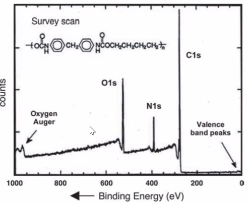
x-ray photoelectron spectroscopy. Ex situ basically just means off-site, so off site investigation of surface composition and structure

Electron spectroscopy for chemical analysis (ESCA) #

Most favorable due to its theoretical strength, sample versatility, and high information content. Similar to auger electron spectroscopy and high-resolution electron energy loss spectroscopy (HREELS). Based on the photoelectric effect: when a photon collides with an electron, all of the energy of the photon is absorbed by the electron and the electron is emitted.

Simplified ESCA experimental setup:

• Material sample is placed in a vacuum and x-rays are directed onto the sample. Atoms in the sample are emitted by core electrons.
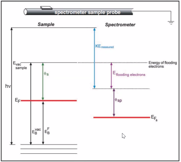
• Photoelectrons are collected and kinetic energy is measured. The magnitude of the kinetic energy contains the binding energy of the electron. Each element has different binding energies for their electrons, so parent element can be identified.
• Relative contribution of different energies can be used to determine the concentration of an element within the sample and morphology of the surface.

When a photon and atom collide, there are three possible events that occur:

• The photon passes through the atom with no interaction
• The photon will lose a portion of its energy due to a collision with an orbital electron (Compton scattering)
• The photon will transfer all of its energy to the orbital electron and eject the electron

Ejections are the important case for ESCA. Photon energy must be sufficient to excite the bound electron. Once electrons start to emit, the number of electrons emitted is a function of intensity of x-ray source and population of the emitting species. Any extra energy over the limit necessary to excite the electron will be added to the electron’s energy in a linear fashion (standard photoelectric effect)

Whe the sample is conductive, then the sample and spectrometer must be grounded together so that they are at the same Fermi level. For insulating materials, reducing space charge effects can’t be done with grounding. Extra electrons must be added to the environment. The energy of the flooding electrons is added to the work function.

Peak width and IMFP (inelastic mean free path): Peak width is equal to planck constant over the lifetime of the vacant hole left by the photoelectron. Peak width are larger for inner electrons and for larger atoms.

IMFP: ESCA is surface analysis, but x-rays can penetrate deep into the sample. Photoelectrons liberated deep within the sample will not make it back to the surface, so ESCA has a limited effective depth..

Inelastic scattering tail: Inelastic electrons will have a higher binding energy.

Auger electron emission peaks: Auger peaks can make it to spectrometer. Small compared to signal, and can be differentiated from the photoelectric peaks by switching x-ray sources.

Degree of vacuum needed depends on sample being examined. Moderate vacuum is fine for most (\( 10^{-6} \) torr), but for reactive samples higher vacuum is needed.

X-ray source: Monochromator limits x-rays projected onto the source to a limited frequency band. Do not want to expose sample directly to x-ray source to avoid noise from Bremsstrahlung electrons.

Electron analyzer: hemispherical electron frequency analyzer splits electrons by energy. Positive and negatively charged hemisphere. The collection lens needs to collect as many electrons as possible to increase signal and protect sample from degradation.

Raman Microscopy #

Need to look this up on my own

Profilometry #

Method of 3D imaging. Fourier transform profilometry (FTP) works by projecting a uniform fringe pattern over an object and then using an image acquisition sensor to record the deformed fringe pattern. The shape of the object can be found by calculating the Fourier transform, filter the spatial frequency, and then calculate the inverse Fourier transform. The height of the object is given by the phase modulation.

Quasi-sine projection and pi-phase shifting technique: Take two pictures of the fringe deformation. Between shots move the grating half a period. This changes the intensity distribution on the object and this method increases the surface slope that can be measured by threefold.

Two dimension fourier transform profilometry: This method helps measure the general shape of a coarse object that has small randomly distributed structures over its surface. The frequency variations of the small structures are attenuated when they are very far away from the carrier frequency of the light. Using a phase and phase unwrapping algorithms will return a 2D continuous function.

Time-delay and integration cameras: TDI cameras are used in FTP to take a 360 degree image of the object and uses a single strip of structured light to find the height distribution on the objects surface.

Reflectivity should not affect the phase modulation, so you get an accurate measurement even if you don’t have a sample of uniform reflectivity.

This is used to determine the surface profile of the cornea when designing contact lenses.

Questions:

• Importance of spectral range of x-ray source? Source must be as monochromatic as possible. Quartz focusing crystal is used to achieve.
• Is the intensity of the transition peak proportional to the abundance of each species? Answer: yes, the cross-section for the absorption is nearly identical for each of the species and the x-ray source frequency is chosen to avoid resonances. The relative abundance of each atomic species appears readily in the intensity ratio (but only for well-calibrated detector!).
• Since they make use of effects in bound electrons, when are XPS/Raman microscopy applicable to plasma experiments? Answer: Ex situ (off-site) measurements are used to investigate samples after the experiment. Examples like titanium oxidized by an O plasma, divertor components, etc.

Infrared Imaging and Two Color Pyrometry - Brett Biggs #

Motivations for optical methods: Many of the methods of plasma diagnostics provide precise data on the composition of the plasma at the cost of directly influencing the state of the plasma

• Often sensors cannot withstand exposure to the extreme temperature
• Noise can be introduced to the system that is difficult to filter - need to isolate sensors electrically or extra post-processing
• Many sensors are required to adequately determine the temperature profile to a sufficient resolution (often interfering with the data you’re trying to collect) - perturbative not great

Optical method features:

• Non-perturbing methods allow various plasma parameters to be directly measured without influencing the plasma.
• IR imaging and two color pyroscopy allow for measurement of the plasma facing components
• Qualitative observations that can predict failure modes

Can be used to diagnose failures in fluid systems - leakage can be readily detected via thermal imaging. Correlation in thermal models to anchor structural models - helpful for determining stresses from CTE, material limits, fatigue, etc..

Why do we care about the temperature in EP devices (such as Hall thrusters)? We care about the life-limiting factors

• cathode insert life is generally a function of temperature
• the anode is greatly impacted by erosion that will degrade thruster performance over time (and cause significant mission impact)
• magnetization will drop as the temperature of the magnet coils increase. Hall thrusters rely upon this magnetic field, will see a significant decrease in efficiency as the magnet coil temperatures rise

IR imaging theory #

What are we measuring? All objects at a temp greater than absolute zero emits photons in the IR range that can be detected.

• Particle motion in warm objects result in charge acceleration or dipole oscillation which produce EM radiation
• In general, the IR emissions from 3 sources will be detected
  • produced by the object due to its temp - some is lost by finite medium transmissibility
  • reflected by the target, sourced by other objects
  • sourced from the medium between the target and camera - vacuum system helps

Camera composition:

• Lens - focuses infrared light from target
• Detector - converts to electric impulse
• Processing electronics
• User interface

Common detectors

• Short wavelength (SWIR): 0.9-1.7 \( \mu m \)
  • InGaAs
• Medium wavelength
  • Indium Antimonide
• Long wavelength
  • SLS
  • HgCdTe
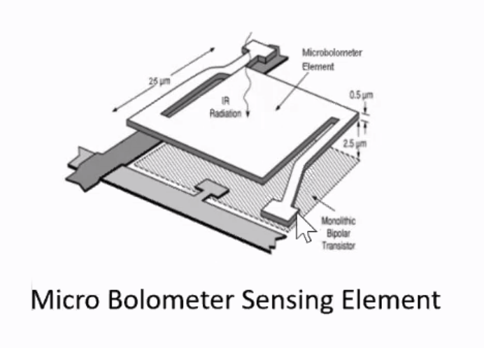
  • Microbolometer

In the study of plasma carrying devices, it is best to use long wavelength detectors for signal clarity - minimize interference between the PFCs and plasma

Cooled Detectors #

• Utilize single photon counting detectors to create the requisite signal for processing. Higher sensitivity than un-cooled detectors
• Cryogenic levels (-200 deg C) must be maintained to avoid blinding the sensor
  • Self irradiance from unit can blind the sensors, making measurements useless
  • Costly to procure and maintain
  • Often significant downtime for maintenance
• Relatively low noise equivalent differential temperature (NEDT)
  • Lower NEDT corresponds to improved resolution
  • Can often resolve 10 mK
• Operating Principles
  • Based on quantum principles. Photoelectric effect raises electrons from valence band to conduction band
  • This changes the conductivity of the material
  • The resulting photocurrent is proportional to the intensity
  • It takes a minimum amount of energy for the photons impacting the detector to elevate the electron from the valence band
  • Peak operating temperature (for camera) higher for shorter wavelength cameras

Un-cooled detectors #

• Photon “masses” required to create signal for imaging electronics
  • Impingement upon resistor laid over large silicon element creates required signal
  • Relies upon bulk change (i.e. temperature) for signal generation
• Higher NEDT than cooled cameras - less sensitive, 30-200mK resolution
• Often provide enough insight into plasma systems to be more useful than cooled systems

Theory #

IR imaging is based off classical equations of heat transfer and photo detection. Materials with non-zero emissivity produce infrared radiation that can be detected by an IR camera. Takes advantage of radiative exchange

Need to define an emissivity to define the emission from a real target. Not constant for any material. In real applications, the rise in temp of the PFCs will alter the emissivity. In applications like EP thrusters, the shift can be measured and is usually small.

The Stefan-Boltzmann equation makes a crucial assumption - that the emissivity over the whole spectral domain (\( \lambda \)) is taken into account. In IR cameras, only a short section of the spectral domain is detected, limiting the effectiveness of the Stefan Boltzmann equation. Instead, the classical definition of the emissivity must be used \[\epsilon(\lambda, T) = \frac{M_\lambda(\lambda, T)}{M_T(\lambda, T)}\]

If we examine the surface of interest in order to determine the temperature, the radiation flux from a surface can be defined as

If we make assumption that surface is Lambertian, radiance is identical in all spatial direction, the photonic flux density is just \( \sin ^2 \theta \Omega \). If we integrate the equations and alter the radiative power equation for a non-blackbody, we find

While true that this is a simplified case, it’s not uncommon in aerospace grade materials. For example, ceramics found in Hall thrusters often are near Lambertian, and can utilized these assumptions.

Over a short range of wavelengths, we can integrate the assumed blackbody photon flux over the spectral domain of interest and multiply by the average emissivity to generate a true photon flux for our measurements

In the case of average emissivity being independent of wavelength, we have what’s called a gray body and we can simplify the calculations.

IR imaging assumptions #

• Assume emissivity is known
• Assume a Lambertian material is being used (simplifying assumption)
  • Non-Lambertian materials don’t prevent measurements from being made, but researcher needs to be wary of curvature
• Imaging device uses wavelength filter to only take in a certain band of spectral range

Limitations #

• Emissivity changes with temperature
  • Can be mitigated by thorough understanding of material
• Emissivity can change with erosion
• Viewing window must be designed to not block IR radiaiton
  • normal glass not compatible, materials such as sapphire glass must be used
  • what other problems will we have even with “compatible” mediums? finite transmission coefficient
  • solution: fiber optic to bypass viewing windows
• Measurement is only as good as your view
  • poor experiment design may prevent critical measurements
• Limited ability to detect wavelengths (single input signal)
• Emissivity can change dramatically with angle of emission - limits measurements of 3D extended bodies where we do not have a normal view of the surface. Really want to be looking at flat features for qualitative assessment. Depending on material properties, increasing angle of incidence may increase or decrease emissivity.
• Emissivity of materials is highly wavelength dependent - depending on range you’re looking at

Two Color Pyrometry #

Need to know the emissivity of the PFCs limit the application of IR imaging. In general, the emissivity of the PFCs will change over time. To overcome limitation, principle is similar to that of single wavelength IR imaging. Two separate signals are ratio’d together.

Planck’s law describes the relationship between radiative intensity and wavelength/temperature. Gives \( u(\lambda, T) \). Simplifying Planck’s law allows us to simplify the model. Assume \( \exp(- C_2/T \lambda) \gg 1 \). In the wavelengths and temps we are interested in, there is generally less than 1 degree difference in model using this simplification.

Two color pyrometry allows us to understand absolute temperature without complete knowledge of the emissivity through all space and time

where \( \sigma_{12} \) is a constant associated with assuming IR emission assuming black body source. It is assumed that the materials will act as a gray-body

• Emissivity is not a function of wavelength
• Deviations from this assumption will increase error

Inverting gives a ratio temperature \( T_r \)

What this indicates is that a temperature can be extrapolated solely from the irradiance of the material being targeted while analyzed to the wavelengths of interest, independent of emissivity. Based on the ratio temperature, some might be wondering how accurate the ratio temperature is. Luckily, it’s simple to extrapolate:

and the temperature error is

Error will stem from the difference in wavelengths being measured. Enter multi-color pyrometry. By taking up to 4 colors allows for higher accuracy measurements to be taken. Higher levels of complexity to resolve additional input signals

• least squares methods common in determining temperature
• Error varies by the precise method being used
• Diminishing returns as the number of wavelengths being analyzed increases, 2 color is common, most don’t go past 4 color

Questions:

• Emissivity measurement error bars are pretty wide (10 percent). What limits this measurement? Answer: Usual way you measure this is by putting your material in an oven and measuring emission with thermocouples, which can be difficult for an entire setup. Additionally, emissivity can change dramatically with angle of incidence, wavelength, etc. So a better way to reduce this error is by computing emissivity ratios by measuring multiple wavelengths (multi-color pyrometry).

Coded Aperture Imaging - Matt Russell #

Technique for imaging high energy x-rays and gamma rays.

Motivated by the lack of a suitable image forming device for x-ray astronomy. By the 1960’s, a pinhole camera was the device by which x-rays were imaged. The pinhole camera projects a 3D image into a 2D plane, with angular resolution determined by the length ratios between the image and source. For a fixed source, this leads to a trade-off between good angular resolution and signal to noise ratio.

Ables and Dicke addressed the problem by introducing a large number of pinholes. The field of view can remain constant while increasing the SNR by having a larger open aperture area - scatter-hole camera.

Linear imaging system #

Linear imaging systems - to first order, let’s consider the imaging system as a linear function from the sensor plane to the detector plane.

\( E(x, y) = S[I(x, y)] \)

if the emitting system can be decomposed into a series of point sources

Rather than measuring the complete linear response, we define an instrument response function (IRF) which measures how the instrument independently responds to each point. We make an assumption that the instrument does indeed respond independently at each point. We also make an isoplantic assumption, assuming that the mapping does not vary over space. This turns the instrument response function into a point source function.

Noise in the system #

• Vignetting
• Blurring
• Distortions
• Diffraction
• Saturation

Add these into a background noise term \( N \)

So, what now? We can remove the correlation between the imaging system and the point source function by taking a Fourier transform. But doing so leads to the Fourier transform of the PSF in the denominator, which contains very small terms that increase the noise. Instead, we can introduce a new re-construction

If we can construct a post-processing correlation function \( G \) such that the correlation between \( A \) and \( G \) is approximately a delta function, then we can remove the correlation without major introduction of noise.

The simplest answer is \( G = A \). This results in autocorrelation and a postprocessing array that is identical to the aperture. This is simple, but there are some problems

• Nonflat sidelobes
• High-frequency fluctuations
• Lack of signal-to-noise improvement

For a coded aperture, we can have a very large (tens of thousands) of pinholes. This means an exact theory for the response of the system would require the response of tens of thousands of pinholes. Mechanically impossible, so use statistics instead.

Questions:

• How far apart are the spacings in the coded aperture in real devices? I assume they have to be much larger than the diffraction range for x-rays (tens of nm). Answer: The imaging grids are usually on the order of a few centimeters, so for a MURA grid with tens of thousands of apertures you’d get grid spacing in the 10-100 micrometer range.

Laser-Induced Fluorescence and TALIF (Two-Photon Absorption) - Aqil Khairi #

Motivation #

Many passive diagnostic methods measure the spectroscopy of plasma self-emission. Now, we induce the plasma excitations with a laser. Bound electrons undergo similar excitation and decay to lower states, and emit radiation. The detected radiation is measured and analysed to obtain certain characteristics of the plasma. The technique is known as Laser-Induced Fluorescence (LIF).

• This can offer a very localized measurement through the crossing of the exciting and viewing beams.
• Species-specific diagnostic; one can tune the laser energy for the desired transition.

LIF has far reaching applications; tumor diagnosis, detection of biomolecules, palentology, and density and velocity measurements of neutral hydrogen in fusion experiments. Neutrals and impurities concentrate in the plasma edge, which is a region of interest especially with regards to PMI at the wall.

Physical Theory - LIF #

Decay from the excited state is on the order of 10ns, so LIF signal depends on the population of excited species. Considered non-perturbing due to short excitation lifetime.

Can stay within this regime by pulsing the laser quickly or maintaining low intensities.

Relationship becomes nonlinear when intensity is so high that ground state ion population is depleted.

Fluorescence from ground state is preferred due to its greater population compared to existing excited states. This helps to avoid saturation.

Physical Theory - TALIF #

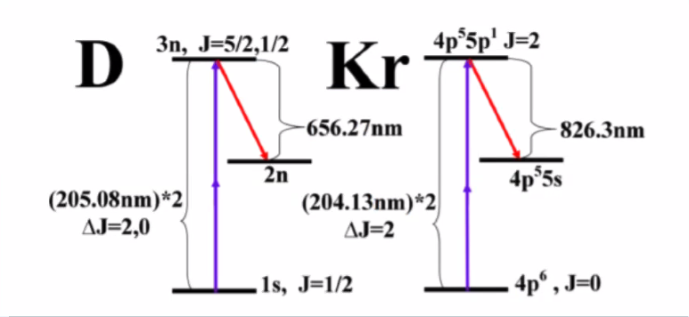
Transmitting UV radiation through windows can be problematic. Fortunately, we can use photons of lower energy and combine them to reach transition energy. Because the fluorescence energy is lower than the excitation, it can be transmitted back through the windows.

In contrast to LIF, the signal is proportional to the square of the laser intensity. This increases the localization of the measurement at the focal point of the beam. Emission as a function of laser wavelength can be used to determine temperature, neutral density, and flow.

Counter-propagation of beams can eliminate Doppler effects. A photon is supplied by each beam, and their Doppler shifts along the beam are equal and opposite.

Physical Theory - Broadening Effects #

Familiar techniques are used to extract temperatures from the observed spectra. Random thermal motion of the particles imparts Doppler shifts to the signal, resulting in Doppler broadening of the line radiation. Before calculating Doppler broadening, you need to take into account a few other effects

• Saturation broadening occurs when the number of excitable particles in the emission volume is exceeded. Not an issue for hydrogen due to rapid decay, but more so in heavier calibration species. One way to expand the linear region is to increase the volume of interest, trade-off in localization.

• Isotopic effects: Energy of atomic states is proportional to the reduced mass (nucleus and electron mass) resulting in a spectral shift. For small atoms, the shift is large and clearly distinguishes isotopes. For higher-mass species, the shift due to isotopic effects is small, but can contribute some artificial broadening.

• Stark broadening: Usually negligible for weak or short-lived electric fields.

• Zeeman splitting: in regions of high magnetic field

• Laser linewidth: can also broaden the signal if it is too large, so the laser system is monitored.

Physical Theory - Signal Dependency #

For TALIF, relationship between emission signal and laser intensity

where

• \( \Delta \Omega \) is solid angle of emission collection
• \( n(v) \) is velocity space density
• \( \sigma \) is absorption cross section for transition
• \( \alpha \) is branching ratio and spectral efficiency of detector
• \( G \) is PMT gain

The wavelength of the laser is scanned to determine the spectral width of the emission.

Omitting the constants and putting in terms of linewidths,

Method #

Development of high energy, narrow spectrum lasers has allowed evolution of LIF to TALIF.

• Dye lasers utilize an organic liquid lasing medium that allows for a wider range of possible wavelengths. Highly tunable, frequency doubling or tripling is possible.
• Pump laser: Provides input energy to the tunable laser. Narrow spectrum to match absorption of lasing medium
• Diode lasers also useful: ubiquitous, can be pumped with current.

Use known pressure of a neutral gas for absolute calibration, e.g. krypton. Krypton is a particularly good choice for calibration because it has a transition very similar in energy to hydrogen and deuterium

Applications #

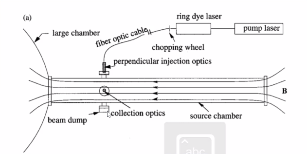
HIT-SI3 Experiment #

• TALIF used for absolute density and temperature measurements of deuterium neutrals
• Frequency tripled dye laser and frequency doubled Nd:YAG laser
• Confocal configuration: Location of measurement controlled by moving focusing lens
• PMT collects emission through a band-pass filter.
• Time resolution achieved through PMT gating.
• Temp, density by fitting measured intensity as laser frequency is scanned.
• Measuring a shift in the centroid of the broadened distribution indicates bulk flow.

MadHex Helicon Plasma Facility #

• LIF setup to diagnose a helicon plasma at Wisconsin using tunable diode laser
• Ion energy distribution function obtained along laser path
• Doppler shift and broadening gives ion velocity and temperature.

Experimental setup showing alignment can look like this:

ITER Divertor #

• Planned LIF configuration for helium density
• Characterization of helium ash removal
• Use Nd:YAG optically pumped dye laser.

Questions:

• You mentioned TALIF measurements of neutral hydrogen in HIT-SI3. Do these LIF measurements have an upper temperature limit once hydrogen is completely ionized, limiting us to early start-up times, or is there still enough neutral hydrogen to fluoresce at operating temperature? Answer: There are still neutrals at the outer edge, but the density decreases as you go deeper into the plasma. In HIT-SI3, they are particularly interested in re-use of hydrogen by liberating neutrals from the wall. In that experiment the focusing lens targets an area very close to the wall in order use TALIF to monitor neutral density/temperature near the wall.

VISAR - Sungyoung Ha #

Fundamentals of VISAR #

VISAR - Velocity Interferometer System for Any Reflector. It is a laser interferometer system for measuring the velocity of a fast-moving surface. Typically used to measure shock propagation or speed of projectiles.

Background of VISAR #

In a Michelson interferometer setup, light from a monochromatic source is split by a beam splitter and travels through two path lengths. If a mirror is moved a distance \( d \) and \( m \) fringes appear/disappear at the center, then \( \lambda = 2 d / m \). How can we use this to measure the speed of a surface? Use the material surface as a mirror for the Michelson interferometer, and count the number of fringes that pass a fixed point.

• Requires a good surface finish for coherent reflection
• Low range of speed measurement (up to a few \( mm / \mu s \))

Another option is to reflect a laser source off the moving surface, causing doppler shifting depending on the velocity. Measuring the doppler shift (knowing the path initial difference) can deduce the velocity. Still requires a very good surface finish, diffusive light will lead to a large intensity difference between legs of the interferometer.

Limitations of Michelson interferometer #

• In practice, the input light is not perfectly collimated and is distributed over an angular range.
• As mirror separation is increased, the spot size (radius from the center to the first minima) decreases. This means that the detector needs to be smaller to properly detect fringes, but this reduces signal strength. Overcome this by a WAMI (Wide Angle Michelson Interferometer) setup.

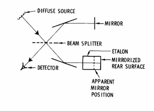
WAMI #

Insert an etalon in one leg of a Michelson interferometer, allows the formation of a virtual mirror closer than the actual mirror. By tuning the apparent position to match the mirror position in the other leg, the detector can see the same image while having a path length difference. The fringe count depends on the amount of the doppler shifted wavelength.

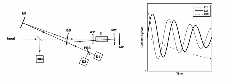
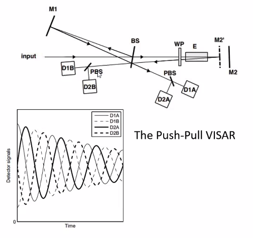
Building on the strengths of WAMI, the VISAR adds:

• BIM (Beam Intensity Monitor) - normalizes the intensity variation of the input (reflected light)
• WP (Wave Plate) - Shifts the phase ofo one polarization by 1/8 wavelengths (total of 1/4 wavelength)
• PBS (Polarizing Beamsplitter) - Splits the output beam

Strengths of VISAR #

• Overcome intensity changes that affect resolution through both design and BIM
• Does not require the surface to be specially treated for reflectivity.
• Good sensitivity and range
• Having two polarized signals with 90 degree phase difference prevents sensitivity loss near the peaks, and allows distinction between positive and negative movement.

Push-Pull VISAR #

A push-pull VISAR setup adds a second detector, utilizing the light lost through the beam splitter.

• Stronger signal strength allows better noise performance, especially in the presence of weak or largely incoherent light.
• Requires additional calibration and balancing.

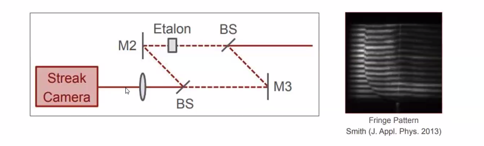
Mach-Zehnder Interferometer version #

Exactly the same as Michelson VISAR, but instead of reflecting through etalon in one leg, the etalon is just inserted into one leg of the Mach-Zehnder interferometer.

Instead of polarizing components, a streak camera is used to obtain a spatial and temporal fringe pattern.

Components of VISAR #

Etalon #

• Fabry-Perot interferometer
• Two partially reflective mirrors separated by a gap. Typically, if the gap is adjustable, it is called an interferometer, and if it is fixed it is called an etalon
• Often used to create interference patterns, filter through certain wavelengths, etc.

Beam Splitter #

• Split beams through half-silvered mirrors of equivalent coating
• Polarizing beam splitters can use birefringent materials, elongated nanoparticles, doped and stretched polymer sheets, Fresnel reflection, or wire gratings to achieve polarization.

Waveplate #

Birefringent (n depending on polarization) material delays a certain polarization state, shifting the phase. Typically made of quartz. Shift depends on material, wavelength, thickness, polarization. Calibrate based on the wavelength of laser you are using. In VISAR setup this can be an issue, since the source is doppler-shifted.

Data interpretation #

Returning to the conventional VISAR setup with two detectors split by 90 degree phase, the normalized components can be expressed as

Because the two polarization states can have different coupling constants throughout the interferometer, we have \( x_0 \) and \( y_0 \). \( \epsilon \) is the phase shift error, or the error from not having an ideal 90 degree phase shift between the two polarization components, including the doppler shift and other various calibration issues.

For \( \phi \) the phase associated with a fringe, we can express it in an elliptic form:

Because we don’t know all of these parameters, but only have a vague understanding of the possible range, we need to perform a fitting of these factors before we can determine velocity data from phase data (fit the ellipses). Usually use iterative numerical schemes to converge to a fitting.

Phase to Velocity #

Once we have the ellipse fitting to interpret the phase data, we need to convert it into velocity data.

Fringe count is just the phase diff divided by \( 2 \pi \) (number of fringes).

Use a VISAR approximation: that the timescale of the event is larger than the delay. Then the approximation can be used to relate the phase and velocity

Corrections and Errors #

• Window corrections (including shocked windows). Typically the surface must be observed through a window.
• Dispersive media (etalon, beamsplitters, etc)
• Fringe uncertainty and ambiguity
• VISAR approximation
• Diffusive reflections
• Multiphase interference

Applications #

Most applications involve high-energy studies.

• Pressure and shock response of materials
• (Hugoniot) Equation of state experiments
• Measure projectile velocity
• ICF: Lasers impinging against the wall of a hohlraum generate shockwaves that compress the deuterium fuel capsule.

Questions:

• What wavelength range is typically used for VISAR? It would seem that there is a trade-off between the velocity resolution (wants longer wavelength) and error correction (wants shorter wavelength). Answer: VISAR setups usually use lasers like Nd:YAG in the visible range. They are readily available and have good signal/noise characteristics for VISAR.

Pulsed Polarimetry - Arvindh Sharma #

What is it #

Pulsed polarimetry is

• A LiDAR like approach to measure the magnetic field and electron density simultaneously.
• A non-perturbative diagnostic best suited for plasmas with high \( n_e \)
• Uses a combination of Thomson scattering and Faraday rotation: when light passes through a plasma, there is some rotation of the polarization
• LiDAR Thomson scattering + polarimetry (measuring the handedness of the polarization of laser light) = pulsed polarimetry
• Used for measuring the parallel component of the magnetic field in a plasma

Principles of Operation #

Three main steps in determining \( n_e \) and \( B_\parallel \)

1. Optical scattering of laser beam by electrons in the plasma (back-scattering). Provides position and number density of the scattering particles
2. Rotation of the polarization azimuth of the probe beam due to \( B_\parallel \).
3. Measurement of time-of-flight and polarization azimuth of the returned laser pulse. The difference in polarization angles when comparing with the reference beam provides information about \( B_\parallel \).

Refresher on LiDAR (Light Detection and Ranging) #

• LiDAR uses laser pulses to detect positions of objects remotely
• It is an active system that supplies energy in the form of laser light
• The reflected light is collected, and the waveform provides useful information about the objects because reflections from more distant objects take longer to return.
• For example, in a plasma, the time difference between peaks would indicate length scales of density variations. The amplitude of the peaks also gives interesting information. A density profile can be constructed from the temporal differences in peaks.

Refresher on polarization #

• Polarization describes the plane in which EM radiation oscillates.
• An EM wave is polarized when the plane of fluctuation of the electric field is well-defined (the plane of fluctuation is perpendicular to the direction of propagation)
• Many natural sources of light are unpolarized
• Laser light is also unpolarized: need polarizers to make it polarized.
• There are 3 types of polarization:
  1. Linear polarization: Electric field oscillates in one plane. Could be the vector sum of linearly polarized components with no phase difference.
  2. Circular polarization: Special case of elliptic polarization where the phase difference is \( \pi/2 \) and the constituent amplitudes are equal. Comes in two flavors: right-handed and left-handed.
  3. Elliptic polarization: Produced by the vector sum of E field components that have different amplitudes and possess arbitrary phase difference. Generic case of polarization.

Optical scattering in pulsed polarimetry #

• Laser pulses are directed through the plasma.
• Electrons produce backscatter radiation through Thomson scattering
  • Thomson scattering is elastic absorption and radiation of EM waves by charged particles.
  • The particles are affected by E and B fields through Lorentz force and oscillate in sync with radiation.
  • The acceleration of the charged particle produces radiation at the same frequency as incoming EM wave.
  • Emitted radiation travels in all directions
• In a range of solid angles around \( \vec k \), the scattering preserves polarization
• LiDAR techniques along with Thomson scattering provide information “local” to the scattering region

Measuring of \( T_e \), \( n_e \), and \( \langle v_e \rangle \) from Thomson scattering #

• Spectrally-resolved scattering intensity is proportional to the electron number density.
• Gaussian broadening provides information about the electron temperature and mean velocity.

Faraday Effect #

• Superposition of left- and right-handed circular polarizations in phas is linearly-polarized light
• In the presence of a magnetic field along \( \vec k \), the right-hand wave propagates faster than the left-hand wave, introducing a phase difference proportional to the index of refraction difference.
• The rotation is proportional to the product of \( n_e B_\parallel \). Also proportional to \( \lambda ^2 \).

Putting it all together #

• The plasma backscattering location is given by \( x = ct / 2 \) where \( t \) is the time of flight.
• The total rotation of polarization azimuth will be twice \( \alpha(I) \) since the light beam travels twice through the plasma: \( \alpha(I, T) = 2.63 \cdot 10^{13} \lambda ^2 \int 0 ^l (n_e B\parallel) [s, t(s)] \dd s \).
• Differentiating \( \alpha \) with respect to path length \( n_e B_\parallel (l) = \left.\frac{1.9 \cdot 10^{12}}{\lambda ^2} \pdv{\alpha_{PP(s)}}{s} \right|_l \)
• In practice, \( \alpha_{PP} \) is plotted as a time series at discrete intervals of \( \Delta T = 2 \Delta L / c \).

Considerations - Laser Pulse Length #

• The spatial resolution depends on the laser pulse length and detection system time scales.
• If detector response time is negligible, then \( \Delta L \) (spatial resolution possible) is \[\Delta L = c/2 \sqrt{ [ \tau_{det} ^2 + \tau_{digitizer} ^2 + (L _{pulse} / c)^2]}\]
• The scattering volume is given by \( \Delta V = \pi r_{beam} ^2 \Delta L \)
• There is a potential trade-off here:
  • To get good spatial resolution, we need \( \Delta L \) to be as small as possible
  • But a short laser pulse might not carry enough energy to induce detectable backscatter or affect SNR
  • Lowering \( \Delta L \) by lowering detector response time adversely affects SNR, since SNR scales roughly as inverse square root of detector band-width.

Considerations - Laser Wavelength #

• Recall that Faraday effect has a square dependence on wavelength of rotation.
• The wavelength needs to be chosen to get detectable resolution of \( \alpha(l, T) \) for smaller path lengths \( l \).
• At the same time, the total rotation through the entire plasma width must not exceed detection range.

Considerations - Time Scales #

• Pulsed polarimetry measures the rotation azimuth on the way to the backscattering location, and on the way back to the detector after scattering
• For this to be true, the plasma conditions need to be “quasi-static” during the laser transit time: must be the same on the first pass as the second pass. In practice this is a very fast time scale and easily satisfied for most plasmas.

Other Considerations #

• The Cotton Mouton effect can be significant in plasmas with strong perpendicular B component.
• The polarization acquires an ellipticity that increases with distance and is quadratic with the intensity of perpendicular B component.
• This effect is due to difference in refractive indices of O- and X-waves.

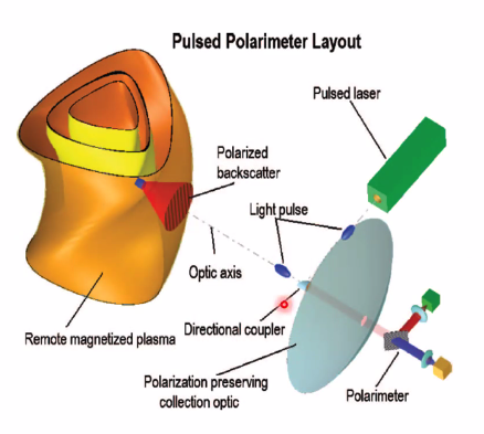
Implementation #

There are 4 major components:

1. Laser source with a spatially narrow, polarized pulse at a chosen wavelength
2. A polarization-preserving collection optic to collimate backscatter from remote plasma locations within a certain solid angle.
3. A directional coupler to redirect laser pulse from source along target optic axis. Don’t want the laser to be looking directly into backscattered light.
4. A polarimeter to detect polarization azimuth and intensity of collected light.

Components: Polarizers #

• Polarizers are used to polarize light in preferred directions
• There are 3 main types: reflective, dichroic, and birefringent
  • Reflective: Surface with a preferential electron direction of motion. Absorb light and reflect light with a well-defined polarization. wire-grid polarizers, Brewster angle polarizers
  • Dichroic: Absorb specific polarization.
  • Birefringent: Different polarizations have different refractive indices.

Components: Polarimeter #

• Polarimeters measure the Faraday rotation and/or electron density
• In amplitude polarimetry, a beam splitter lets original polarization pass and reflects orthogonal component. The Faraday rotation induces the orthogonal component. The reflected beam is combined with a frequency-shifted reference beam. The amplitude of the heterodyne beat is proportional to the Faraday rotation.

Applications (proposed) #

• FRX-L plasma
  • Experiment at LANL
  • Uncompressed FRC
  • 50 GW Nd:YAG laser suggested
  • \( L_{pulse}/c = 20 ps \)
  • 10 pulses at 100mJ/pulse
• FRCHX plasma
  • Experiment at Kirkland AFB device
  • Compressed FRC
  • 100 GW tripled Ti:sapphire laser
  • \( L_{pulse}/c = 1 ps \)
• ITER
  • Challenging because of low electron density and magnetic field
  • A far infrared laser source needed
  • Pulsed polarimetry could provide real-time control to prevent MHD instabilities

In-use application: University of Washington Pulsed Polarimeter was modified to sense magnetic field using a streak camera and fiber optic PP (Smith and Weber, 2016).

Advantages #

• Measures local magnetic field using a remote, non-perturbative method
• Spatial resolution of millimeters on high energy density plasmas
• Can simultaneously measure \( T_e \), \( n_e \), and \( B \) along line of sight.
• Resilient to refractive effects and short measurement duration, so can be used to control instabilities.

Summary #

• Pulsed polarimetry is a LiDAR-like technique that incorporates Thomson scattering with Faraday rotation
• It is proposed to be a peerless technique for remotely sensing magnetic field in plasmas
• With the right choice of optical components and energy sources, it can aid in real-time control of experiments to address instabilities.
• Technology is still nascent - lots of potential for future applications.

Questions:

• How are we able to get spatially-resolved information about the parallel magnetic field strength when the Faraday rotation is going to be line-integrated along the line of sight? A: The rotation is cumulative over the path of travel, so we get a cumulative distribution over the path. If we can compute the local \( n_e \) along the path, we can differentiate to recover the local magnetic field.

LIDAR Incoherent Thomson Scattering - Josh Perry #

Pulsed Thomson scattering is one of the essential elements of pulsed polarimetry. Used to determine temperature and density of electrons. There are limitations to other methods of getting these diagnostics:

• Langmuir probes: perturbative
• interferometry: line-integrated
• Spectroscopy of line radiation: indirect

Thomson scattering is direct, weakly-perturbing, and localized

Overview #

Light from a laser source scatters off electrons in the plasma. Temperature is determined from the doppler broadening of scattered light. Density is determined from the absolute intensity of scattered light. Measurements are localized to the intersection of laser and viewing beams

Scattering Theory #

For \( h \lambda \ll m_e V_e \), quantum effects can be ignored. This is the difference between Compton scattering (quantum) and Thomson scattering (classical). The electron oscillates in the wave fields, giving off radiation from its acceleration. When the Debye length is much greater than \( \lambda \), incoherent scattering.

Doppler shifting of scattered radiation is only in the \( \vec k \) direction. At high temperatures (1keV), relativistic effects shift towards blue, making temperature seem higher.

Density determined from scattering cross-section

The cross-section is small, and for high spatial resolution the scattering volume is small, so very high intensity laser required. Calibration performed using a neutral gas.

Noise Sources #

• External sources: any stray light can be an important noise source, since the scattered intensity is low. Blocking sightlines, covering windows, and using viewing dump can help reduce external noise.
• Stray laser radiation: self-absorption of laser source. Narrow bandwidth makes it easy to identify in spectrum. Use beam dump to reduce noise.
• Line radiation from plasma. Avoid coincident lines by adjusting laser frequency if using tunable laser.
• Bremsstrahlung: most unavoidable noise source

For polarized laser, polarimetry can be used to reduce noise.

Types of Thomson Scattering Setup #

Perpendicular Thomson Scattering #

• Simplest and most common TS configuration. Viewing and laser beams are orthogonal, scattering volume limited to a relatively small region

TV Thomson Scattering #

Use a group of lenses to gather scattered light from multiple locations along one or more laser beams. Forms a 2D image at the spectrometer detector. High complexity due to many optical paths.

LIDAR Configuration #

Laser and detector optics are located on same port, measuring backscattered radiation. The time of flight depends on the plasma depth, allowing for spatial resolution along flight path. Requires extremely short laser pulse. LIDAR systems used in large tokamak experiments (ITER, JET).

Questions:

• Do you know what limits the repeatability of LIDAR TS? 0.5 Hz doesn’t give you very many data points in a single shot. In very high-intensity lasers, what tends to limit the repeatability is the process of the lasing medium de-exciting back to the ground state. This takes much longer than any other process in the collection setup.

Coherent Thomson Scattering - Simon Fraser #

When Thomson scattering occurs in the limit that \( k \lambda_D \ll 1 \), collective effects become dominant and we all the phenomenon coherent Thomson scattering (CTS). CTS diagnostic is a non-perturbative measurement that provides information on the electron density, electron temperature, ion temperature, and flow velocity. CTS has very good spatial and temporal resolution and has been used in systems ranging from Hall thrusters to fusion confinement experiments.

What is Thomson scattering? #

Thomson scattering is elastic scattering of EM radiation by a free charged particle. It is also the low energy limit of Compton scattering. Ignores relativistic effects, applicable for \( T_e < 1 keV \)

The process goes like this

• EM radiation approaches a free particle
• The particle moves in the electric and magnetic fields of the EM wave
• The movement of the free particle creates an EM wave
• Scattered in all directions; direction of interest determined by line of observation

What is coherent (collective) Thomson scattering? #

• Scattering calculations in a plasma involve electric field contributions from many electrons. In incoherent Thomson scattering, the collective effects of the plasma can be ignored and all contributions are assumed to be uncorrelated. Coherent Thomson scattering is the case where the contributions from separate particles are correlated.
• Recall that electrons shield each other on the order of the Debye length. If \( k \lambda_D \gg 1 \) then the phase difference between the scattering resulting from an electron or its shielding cloud is large. The scattered radiation is then incoherent.
• If \( k \lambda_D \ll 1 \) then the phase difference is small, and the scattering off of an electron is balanced by the absence of scattering from its shielding cloud. Scattering from ions is negligible (factor of \( m_e/m_i \)).
• Recall that \( k \lambda_D \ll 1 \) is equivalent to \( 2 \pi \lambda_D \ll \lambda \). Sometimes given in terms of a scattering parameter \( \alpha = 1/k \lambda_D \).

Use as a plasma diagnostic #

• Scattered field from a single electron

with classical electron radius \( r_e \), tensor polarization operator \( \vec \Pi \), and distance to observer \( R = x - \vu s \cdot \vec r \) where \( x \) is position of observation. From a population of electrons,

with Klimontovich point distribution function \( F_e \). For monochromatic incident light, the total scattered power is

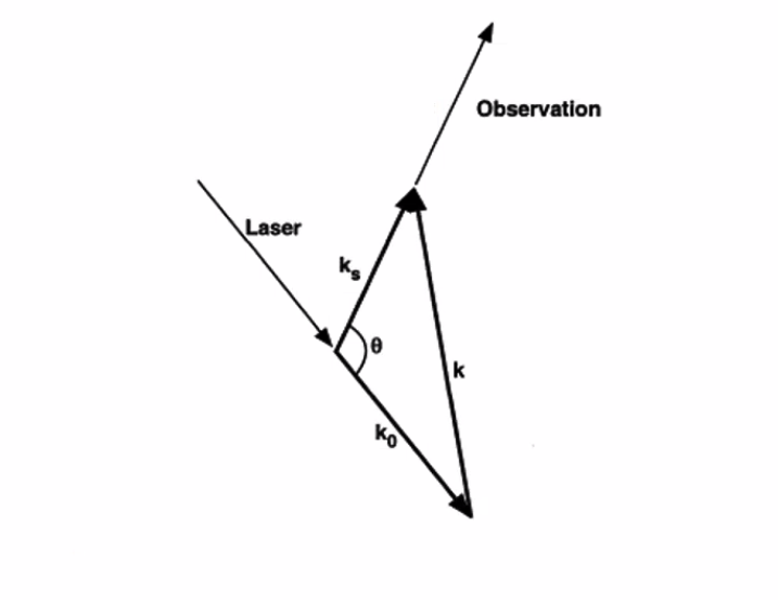
with \( r_0 = e^2 / m_e c^2 \) and \( |\vu s \cross (\vu s \cross \vu E_i) = 1 - \sin ^2 \theta \cos ^2 \beta \) where \( \theta \) is detection angle and \( \beta \) is the angle of the incident polarization vector relative to the scattering plane and \( L \) is the length of the Thomson scattering volume. Notably, incident polarization perpendicular to the scattering plane gives the strongest signal.

Collective ion-acoustic features can be observed, as long as \( Z T_e / T_i > k_a ^2 \lambda_D ^2 \). This means that the electrons follow the motion of the ions. In this regime the scattering occurs from co- and counterpropagating ion-acoustic waves.

The wavelength separation between the ion-acoustic features is

\( \Delta \lambda / \lambda_0 \) is often very small.

Doppler shift #

The Doppler shift of the scattered radiation contains information about the bulk velocity.

Note that charges parallel to the incident light get the maximum shift.

Diagnostic calculations #

Temperature of electrons and ions can be derived by fitting the observed spectrum to the appropriate form factor.

Electron density can be determined through the total scattered power, the frequency of the electron plasma wave, or two-color Thomson scattering. The two-color approach relies on the difference between the ion acoustic frequency at large and small k-vector values. The small k-vector fluctuations provide electron temperature while large k-vector fluctuations provide the density. This can be done with a single laser and different scattering angles.

Note that \( k \) increases with both frequency and angle of incidence.

Detection angle \( \theta \) considerations:

• 90 degress is convenient: reduces stray light and gives best measurement localization
• greater than 90 degrees is backscattering, less than 90 degrees is forward scattering
• Detection angle affects whether the scattering observed is coherent or incoherent; behavior is more collective at small \( \theta \).

Laser considerations:

• Laser frequency must be greater than the plasma frequency to avoid heating
• Laser pulse energy should also be tuned to avoid heating
• Scattering signal is most intense for a laser polarized perpendicular to the plane of the laser beam and observation direction
• Shorter pulses increase SNR and temporal resolution
• Wave resonances need to be avoided to avoid heating

Sources of error

• Plasma self-emission
• Stray light
• Rayleigh scattering background
• Broadening effects
• A more powerful laser increases signal-to-noise ratio

Use in experiments #

• Diagnosing Hall Thruster instabilities (PRAXIS)

  • Propulsion analysis experiment via infrared scattering
  • Uses 10.6 \( \mu m \) \( CO_2 \) laser split into two beams, primary and local oscillator
  • Local oscillator is a reference beam to get phase and amplitude information
  • Local oscillator gets mixed with scattering signal
  • Very highly localized measurement determined by interference between the two beams

• ASDEX tokamak

  • Uses CTS to measure ion velocity, ion temp, and ion composition
  • Here, magnetic vector perpendicular to the wave vector, so can observe the effects of ion Bernstein wave
  • Uses 2ms pulses

Questions:

• You mentioned experiments using both continuous and pulsed laser systems. Did you come across any configurations that used LiDAR-like ranging schemes for spatial resolution? Answer: Did not come across any configurations that used ranging schemes to spatially resolve. The time scale over which ion-acoustic affects occur may be too long compared to the time of flight to obtain meaningfully resolved ion temperature/density measurements.