Zeeman Spectroscopy #

Motivation #

In high-energy-density plasmas, the current density distribution is strongly tied to the magnetic field distribution, and in some regions measurement of the B-field is the only way to obtain current density measurements. The magnetic field also determines resistivity, plasma dynamics, and energy balance.

The diagnostic methods to measure localized magnetic fields in plasma make use of the Zeeman effect, the Stark effect, Faraday rotation, or Faraday’s law. Each method has benefits/drawbacks that need to be taken into account. Some provide chord-integrated measurements, some spatially resolved. Physical probes can perturb the plasma you are trying to measure, or be destroyed in a plasma-facing environment. Zeeman spectroscopy is a non-perturbative, passive diagnostic. The extent of spatial and temporal resolution and error is highly dependent on the experimental setup.

Zeeman Splitting #

The Zeeman effect is the effect of a magnetic field on the states of a bound electron. Discovered by Pieter Zeeman in 1896 when there was very little understanding of quantum mechanics, it was the subject of the 1902 Nobel prize. It was discovered that spectral lines seemed to split in a magnetic field, and the satisfactory explanation had to wait until the development quantum mechanics. A bound electron has two magnetic moments, one associated with the orbital motion

and the magnetic moment due to the spin

the classical Hamiltonian of this magnetic moment interacting with an external magnetic field \( \vec B \) is

where \( \hat \mu \) is the magnetic moment of the electron, \( m_e \) is the electron mass, \( c \) is the speed of light, \( \hat L \) is the angular momentum operator, \( \hat S \) is the spin operator, and \( \vec B \) is the externally-applied magnetic field we wish to measure. By convention, we choose the z direction to align with \( \vec B \). This term is treated as an addition to the “un-perturbed” Hamiltonian

Things would be rather simple without incorporating the fine structure term, but alas we cannot discount it entirely. In the fine structure term, there is something like an internal magnetic field in the atom which is responsible for the spin-orbit coupling term. We can treat separately the cases where the external magnetic field is either much smaller or much larger than this internal magnetic field. In the weak case, we treat \( H_{Zeeman} \) as a perturbation atop the result of the fine-structure states. In the strong case, the Zeeman effect is assumed to be much stronger than the spin-orbit coupling, so we then take the fine structure Hamiltonian as a perturbation atop \( H^{(0)} + H_{Zeeman} \). For the fields which we wish to measure in plasma diagnostics, it is the “weak” Zeeman effect which generally applies. In the “strong” Zeeman effect, known as the Paschen-Back effect, the spin-orbit coupling is broken by the externally applied field, and the line splitting reverts to the normal (total spin 0) Zeeman effect.

For the weak effect, we calculate the expectation values of the perturbing Hamiltonian, which will add to the known energy levels:

As it turns out, this product is completely diagonalizable and the energy level splitting is given by:

\[\langle \psi | L_z + 2 S_z | \psi \rangle = \frac{g_J m_j}{\hbar}\] \[E_{Zeeman} = g_J \mu_B m_j B\]

where \( g_J \) is the Landé g-factor \[g_J = 1 + \frac{ j (j+1) + s (s+1) - l (l+1)}{2 j (j+1)}\]

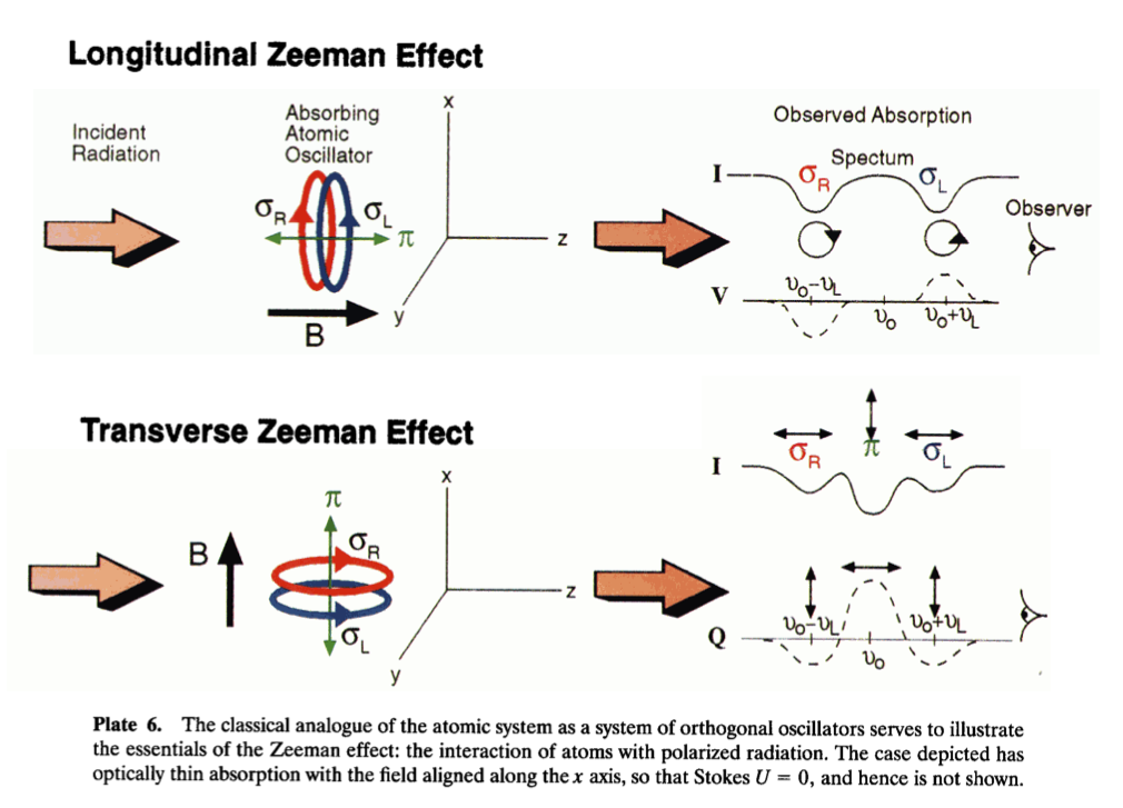
and \( \mu_B = \frac{e \hbar}{2 m_e c} \) is the Bohr magneton. Two features are of key importance: First, the energy level splitting is proportional to \( B \), inviting a measurement of the field by a direct observation of the level splitting. Unfortunately, for most applications the Doppler and Stark broadening are an order of magnitude greater than the Zeeman splitting. Fortunately, conservation of angular momentum gives us another useful property: the polarization of the emitted radiation is dependent on \( \Delta m \) (the projection of the total angular momentum in the direction of \( \vec B \)). Emission is only possible for transitions for which \( \Delta m = [-1, 0, 1] \). The components for which \( \Delta m = 0 \) are called the \( \pi \) components, and the components for which \( \Delta m = \pm 1 \) are the \( sigma \) components. When emission is viewed parallel to \( \vec B \), only the \( \sigma \) components are observable and the emission is circularly polarized, right handed direction for \( \Delta m = +1 \) and circularly polarized, left handed for \( \Delta m = -1 \). When viewed perpendicular to \( \vec B \), the emission is linearly polarized, with \( \pi \) components polarized parallel to \( \vec B \) and the \( \sigma \) components polarized perpendicular to \( \vec B \). Since the Doppler and other broadening effects do not change the polarization of the light, these properties allow for resolution of the Zeeman splitting in the presence of substantial broadening using polarization discrimination techniques.

[https://doi.org/10.1029/1999RG900011]

Low-density magnetic field measurement #

Early (1989) spectroscopic measurement of the magnetic field in a low-density (\( \sim 10^{15} cm^{-3} \)) plasma was carried out by directly measuring the Zeeman splitting in a high-power diode plasma [PhysRevA.39.5856]. At low density high temperature, the Doppler broadening is the main broadening effect. The Zeeman splitting can overcome the Doppler broadening by observing the splitting of long-wavelength emissions (the Zeeman splitting is proportional to \( \lambda _0 \)) from heavier ions, in this case Ba-II.

Measurements of magnetic field in Z-pinches #

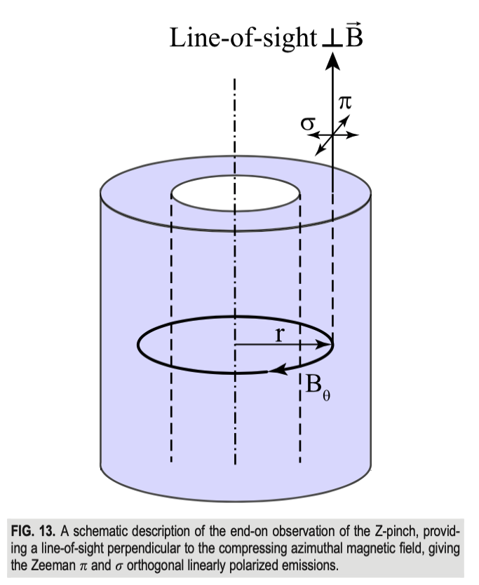
In a Z-pinch configuration, the magnetic field has a well-defined (azimuthal) direction, and polarization techniques can be used to resolve the Zeeman splitting even when smeared by Doppler and pressure broadening. With a magnetic field of known direction, we have a choice between measuring emissions parallel to the field direction (perpendicular to the axis of symmetry) or perpendicular to the field direction (“end-on” measurements). In the cylindrical geometry, this decision amounts to choosing between chord-integrated and radially-resolved measurements.

End-on observations #

Observing the splitting of line emission end-on allows for radially-resolved measurements:

[doi:10.1063/5.0009432]

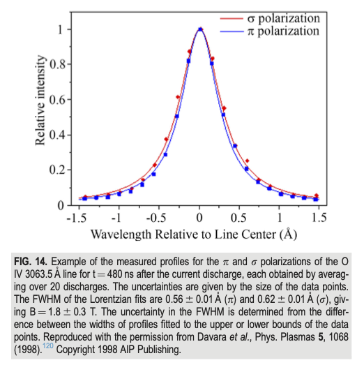
The polarization of Zeeman-split emission perpendicular to the magnetic field is linearly polarized, and both \( \pi \) and \( \sigma \) components are visible. This was the method used in one of the first measurements of the B-field in a Z-pinch experiment [doi:10.1063/1.872637]. The \( \sigma \) and \( \pi \) components are orthogonally polarized, so they can be distinguished by the use of linear polarizers. The \( \sigma \) components have the same polarization, so they cannot be separated from each other by polarizers. A fit of the broadened line can be obtained for each polarization direction, assuming identical broadening parameters (temperature, pressure, etc.). The difference between the spectral linewidths is proportional to the magnitude of the magnetic field. In general, the linewidth difference is very small, and the diagnostic requires a very high signal/noise ratio. In this experiment, such a signal/noise ratio required averaging over many discharges, so this measurement is highly dependent on shot reproducibility. Stark and Doppler broadening also limit the applicability of the method; at small radius and high pressure, the linewidth difference becomes too small to determine.

[doi:10.1063/5.0009432]

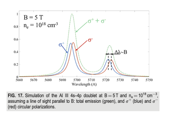
Vertical observations (Two-polarizations method) #

For a line of sight parallel to the magnetic field, only the circularly polarized \( \sigma^+ \) and \( \sigma ^- \) components are visible. By combining a quarter-wave plate and a linear polarizer, we can obtain separate broadened lines for the \( \sigma^+ \) and \( \sigma^- \) components. The Doppler and Stark broadenings are polarization independent so identical fitting parameters are used for each line. Calculating the separation between the centroids gives a more reliable measurement, less sensitive to noise. Of the Zeeman splitting diagnostic methods, this has the highest sensitivity to B since it relies on the line positions rather than their shapes.

[doi:10.1063/5.0009432]

In a cylindrical geometry like a z-pinch, at first glance it appears that we can only obtain a single measurement along the chord at the outer-most radius of the plasma extent. At other positions, the magnetic field is not parallel to the line of sight, so the emission is elliptically polarized. This has the effect of lowering the perceived Zeeman shift, since the transverse components appear as un-shifted lines. We could perform an Abel inversion of the chord-integrated measurements to recover the radial magnetic field distribution, but in most imploding plasma experiments there is a lack of sufficient azimuthal symmetry and Abel inversion gives misleading results.

There is a significant radial temperature gradient in a z-pinch. For the most part, impurities burn through at well-defined temperatures, resulting in a radial distribution of impurity species. In shells closer to the symmetry axis, lower ionization states become ionized. This allows us to select emission lines specific to the various impurity species, and “see through” the outer shells by observing emission lines not present in the outer shells. If the radial distribution of impurity species is known, the radial distribution of the magnetic field can be resolved without the need for Abel inversion.

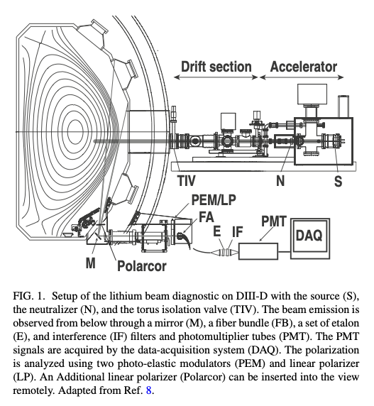
Neutral beam injector #

Zeeman spectroscopy can be achieved with the help of neutral beam injection. This is particularly useful in a configuration in which large populations of impurity species are highly undesirable, or when large intrinsic radial electric fields preclude the use of the motional Stark effect (MSE). In a neutral beam injection diagnostic, a beam of neutral atoms (\( \sim 30keV \) beam energy) is injected into the plasma. The beam becomes excited by collisions with the plasma, emitting characteristic line radiation which is split by the magnetic field. Because the beam is neutrally charged, the beamline is not altered by the presence of the strong magnetic field in the plasma. The beam continues through the plasma to a beam dump opposite the injector. The optical setup is arranged vertically, perpendicular to the beam injection, in order to obtain radially-resolved measurements with maximum sensitivity to the longitudinal magnetic field.

Considerations for the neutral beam injector:

• The beam should be of a high enough energy to penetrate well into the plasma. The beam penetration determines the radial extent of the measurement.
• Extremely low intrinsic ion temperatures are preferable. Doppler broadening is the main obstacle to overcome in resolving the Zeeman splitting, and beam temperature is a major contributor to the linewidth. Sources of intrinsic ion temperatures of \( \sim 0.1 eV \) have been demonstrated in use.
• The beam current must strike a balance between signal strength and perturbation of the plasma. An extremely low beam current will not produce sufficient line emission, but an excessive beam current has the potential to disrupt the system under study.
• A tightly focused beam improves the volumetric resolution.

[doi:10.1063/1.1526928]

With a sufficiently high signal/noise ratio, the direction and magnitude of the magnetic field can be determined. For example, in the DIII-D diagnostic configuration shown here, the ratio of circular to linear polarization in the \( \sigma^- \) line is sufficient to determine the direction of the magnetic field.

Pros:

• High spatial resolution
• Applicable even when direction of magnetic field is not known

Cons:

• Neutral beam injector itself is a substantial addition to the experimental setup. Beam injector requires its own set of diagnostics.
• Can be perturbative, depending on beam strength

Pellet injection and laser blow-off are alternate methods of injecting impurity species. Pellet injectors are common in tokamaks for fuel injection during operation. They can also be used to inject pellets of impurity species for the purpose of spectroscopy. A pellet is launched into the plasma, where it vaporizes. The ablation cloud emits line radiation, which can then be analyzed for Zeeman splitting. Used in TFTR and others. In a laser blow-off setup, ions can be injected at the plasma edge by preparing a thin film on a glass plate, then blasting it off into the plasma chamber with a laser. Used in Wendelstein 7-X and others.

Remote sensing of solar magnetic field #

For extraterrestrial plasmas, the only diagnostics available are spectroscopic. Investigation of the solar magnetic field lead to the early development of polarimetric techniques for the measurement of Zeeman splitting. The Zeeman effect provides the most common and useful diagnostic of solar magnetic fields [https://doi.org/10.1029/1999RG900011]. The spectral shapes of emission and absorption lines are altered by the solar magnetic field, and circular and linear polarization are imparted according to the direction of the field. Analysis of the absorption and emission spectra requires assumptions about the structure of the solar atmosphere. Neutral iron (Fe I) is a particularly good source of data about sunspots, as ferromagnetic atoms are especially Zeeman-sensitive and the long-wavelength 630.2 nm absorption lines enhance the splitting effect. By decomposing the polarization of absorbed emission, the direction and strength of the solar magnetic field can be recovered. This is how it was discovered that sunspots are regions of high magnetic flux; weak magnetic fields away from sunspot, then suddenly when you look at the spot the lines split.