Real Integrals #

In real life, we often want to evaluate real integrals, which is to say we want to integrate a real-valued, single-valued function along the real axis. Numerically, this is pretty straightforward to do using a Riemann sum, although it can become difficult if the function goes to zero very slowly.

We can turn a real integral into a complex contour integral by appropriately choosing a contour in the complex plane such that one segment of the contour corresponds directly with the real integral, and the remaining segment can be evaluated (usually as 0) leaving us with a closed contour integral.

Suppose we want to evaluate

We can turn this into a contour integral over the upper half plane (or lower half plane) and taking the limit as \( R \rightarrow \infty \):

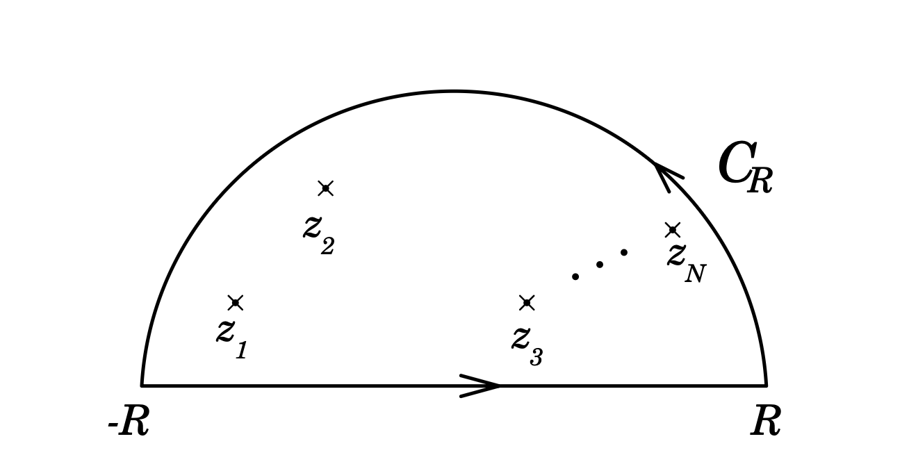
where \( C_R \) is a large semicircle and the contour encloses all singularities of \( f(z) \). Along \( C_R \),

If we can show that \( |z f(z)| \rightarrow 0 \) as \( |z| \rightarrow \infty \), then the \( C_R \) contribution goes to zero. We can use Cauchy’s residue theorem to evaluate the closed contour integral:

We could also choose the lower half-plane, as long as we remember to keep the minus sign as \( \theta \) would be going clockwise there.

Example

For any positive integer \( N \). First, we want to extend this to cover the whole real axis so that we can close the contour. Since the integrand is even,

Then, we need to check that the contribution from the \( C_R \) contour will be zero

We can bring out the reverse triangle inequality here:

\[\left| z \frac{1}{1 + z^N} \right| \leq \frac{|z|}{|z|^N - 1} = \frac{1}{|z|^{N-1} - \frac{1}{|z|}}\] \[\lim_{z \rightarrow \infty} \frac{1}{|z|^{N-1} - \frac{1}{|z|}} = 0\]

Okay, at this point we can proceed to find the residues:

At this point we can quote the residue theorem to say

The simple poles of our \( f(z) \) occur where \( 1 + z^N = 0 \)

\[z^N = -1 = e^{i (\pi + 2 \pi k)}\] \[z = e^{i \frac{\pi + 2 \pi k}{N}} \quad k = 0, 1, \ldots, \frac{N}{2} - 1\]

We can use the differentiation trick above to find the residues of the simple poles:

Example: Improper integral of an odd rational function

Evaluate

Because we have an integral on \( 0, \infty \), we can’t immediately close the contour using \( C_R \) as shown above. We also can’t expand the integral to the whole real axis because \( f(x) \) is not an even function.

However, there is a useful symmetry we can apply here: \( (x e^{2 \pi i / 3})^3 = x^3 \). This suggests using the following contour, where \( C_R \) is the sector \( R e^{i \theta} : 0 \leq \theta \leq 2 \pi / 3 \):

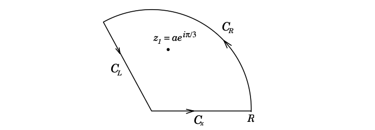
We therefore have:

The only pole inside \( C \) satisfies \( z^3 = - a^3 = a^3 e^{i \pi} \) and is given by \( z_1 = ae^{i \pi / 3} \).

The residue is obtained from

The integral on \( C_L \) is evaluated by making the substitution \( z = e^{2 \pi i / 3} r \) (where the orientation is taken into account)

Thus taking into account the contributions from \( C_x \) (\( 0 \leq z = x \leq R \) ) and from \( C_L \), we have

Thus

Trigonometric Integrals over a Period #

For another example, consider an integral of some trigonometric function over a full period:

where \( U \) is some annoying-to-integrate function like \( \sin ^2 \theta / (a + \cos \theta) \). We can turn it into a closed contour integral over the unit circle where

\[z = e ^{i \theta} \qquad 0 \leq \theta < 2 \pi\] \[\dd z = i e^{i \theta} \dd \theta = i z \dd \theta \rightarrow \dd \theta = \frac{\dd z}{i z}\]

From there, we can re-parameterize \( U \) using

\[\cos \theta = \frac{1}{2} (e ^{i \theta} + e^{-i \theta}) = \frac{1}{2} (z + \frac{1}{z} )\] \[\sin \theta = \frac{1}{2i} (e^{i \theta} - e^{-i \theta}) = \frac{1}{2i} (z - \frac{1}{z})\]

For example, if we have

then the integral becomes

The simple poles of the integrand are where \( z^2 + 4iz - 1 = 0 \), and these are found at

Of those, only \( z_1 \) is found within the unit circle, so

To find the residue, re-express the integrand using the roots:

and then multiply by \( (z - z_1) \):

\[\text{Res}[z_1] = \lim_{z \rightarrow z_1} \frac{(z - z_1) 2}{(z - z_1)(z - z_2)} \\ = \frac{2}{z_1 - z_2} = \frac{1}{i\sqrt{3}}\] \[I = 2 \pi i \left( \frac{1}{i\sqrt{3}} \right) = \frac{2 \pi}{\sqrt{3}}\]

It is sometimes convenient, when analyzing the behavior of a function near infinity, to make the change of variables \( z = 1/t \). Using \( dz = - \frac{1}{t^2} dt \) and noting that the clockwise (positive direction) of \( C_R: z = R e^{i \theta} \) transforms to a clockwise rotation (negative direction) in \( t \): \( t = 1/z = (1/R)e^{-i \theta} = \epsilon e^{-i \theta} \) we have

where \( C_{\epsilon} \) is the limit as \( \epsilon \rightarrow 0 \) of a small circle around the origin in the \( t \) plane. So the residue at \( \infty \) is given by

that is, the right-hand side is the coefficient of \( t^{-1} \) in the expansion of \( f(1/t)/t^2 \) near \( t = 0 \); the left-hand side is the coefficient of \( z^{-1} \) in the expansion of \( f(z) \) at \( z = \infty \) . Sometimes we write

The concept of residue at infinity is quite useful when we integrate rational functions. Rational functions have only isolated singular points in the extended plane and are analytic elsewhere. Let \( z_1, z_2, \ldots, z_N \) denote the finite singularities. Then, for every rational function,

[]

Theorem

Let \( f(z) = N(z) / D(z) \) be a rational function such that the degree of \( D(z) \) exceeds the degree of \( N(z) \) by at least two. Then

\[\lim_{R \rightarrow \infty} \int_{C_R} f(z) \dd z = 0\]

We write

\[f(z) = \frac{a_n z^n + a_{n-1} z^{n-1} + \ldots + a_1 z + a_0}{b_m z^m + b_{m-1} z^{m-1} + \ldots + b_1 z + b_0}\]

Then, by repeated application of the triangle inequality,

\[\left| \int_{C_R} f(z) \dd z \right| \leq \int _0 ^\pi (R \dd \theta) \frac{ |a_n| |z|^n + |a_{n-1} | |z| ^{n-1} + \ldots + |a_1| |z| + |a_0|}{|b_m||z|^m - |b_{m-1}| |z| ^{m-1} - \ldots - |b_1| |z| - |b_0|} \\ = \frac{\pi R(|a_n| R^n + \ldots + |a_0|)}{|b_m| R^m - |b_{m-1}| R^{m-1} - \ldots - |b_0|} \rightarrow _{R \rightarrow \infty} 0\]

since \( m \geq n + 2 \)

Some integrals that are closely related to the one described above are of the form

\[I_1 = \int _{-\infty} ^{\infty} f(x) \cos (kx) \dd x\] \[I_2 = \int _{-\infty} ^{\infty} f(x) \sin (kx) \dd x\] \[I_{3 \pm} = \int_{-\infty} ^{\infty} f(x) e^{\pm ikx} \dd x \qquad (k > 0)\]

where \( f(x) \) is a rational function satisfying the conditions of the theorem above. These integrals are evaluated by a method similar to the ones described earlier. When evaluating integrals such as \( I_1 \) or \( I_2 \), we first replace them by integrals of the form \( I_3 \). We evaluate, say \( I_{3+} \) by using the contour \( C_R \) above. Again, we need to evaluate the integral along the upper semicircle. Because \( e^{ikz} = e^{ikx} e^{-ky} \), we have \( |e^{ikz}| \leq 1 \) (where \( y > 0 \) ) and

from the results of the theorem. Thus using

By taking the real and imaginary parts, we can compute \( I_1 \) and \( I_2 \)

Example

Evaluate

We consider

and use the contour \( C_R \) shown above to find

From

we have

and

If \( b = 0 \) the latter formula reduces to \( J = 0 \), which also follows directly from the fact that the integrand is odd. The reader can verify that

In applications we frequently wish to evaluate integrals like \( I_{3\pm} \) involving \( f(x) \) for which all that is known is \( f(x) \rightarrow 0 \) as \( |x| \rightarrow \infty \). From calculus we know that in these cases the integral still converges, conditionally, but our estimates leading to

must be made more carefully. We say that \( f(z) \rightarrow 0 \) uniformly as \( R \rightarrow \infty \) in \( C_R \) if \( |f(z)| \leq K_R \), where \( K_R \) depends only on \( R \) (not on \( \text{arg}(z) \) ) and \( K_R \rightarrow 0 \) as \( R \rightarrow \infty \). We have the following lemma, called Jordan’s Lemma

Jordan’s Lemma #

\[\]

Jordan’s Lemma

Suppose that on the circular arc \( C_R \) shown above, we have \( f(z) \rightarrow 0 \) uniformly as \( R \rightarrow \infty \). Then

\[\lim_{R \rightarrow \infty} \int_{C_R} e^{ikz} f(z) \dd z = 0 \qquad (k > 0)\]

With \( |f(z)| \leq K_R \) where \( K_R \) is independent of \( \theta \) and \( K_R \rightarrow 0 \) as \( R \rightarrow \infty \),

\[I = \left| \int_{C_R} e^{ikz} f(z) \dd z \right| \leq \int_{0} ^\pi e^{-ky} K_R R \dd \theta\]

using \( y = R \sin \theta \) and \( \sin(\pi - \theta) = \sin \theta \)

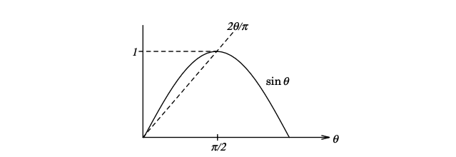
\[\int_0 ^\pi e^{-ky} \dd \theta = \int_{0}^\pi e^{-kR \sin \theta} \dd \theta = 2 \int_0 ^{\pi / 2} e^{-k R \sin \theta} \dd \theta\]

But in the region \( 0 \leq \theta \leq \pi / 2 \) we also have the estimate \( \sin \theta \geq 2 \theta / \pi \)

Thus

\[I \leq 2 K_R R \int_0 ^{\pi / 2} e ^{-2 k R \theta / \pi} \dd \theta = \frac{2 K_R R \pi}{2kR} (1 - e^{-kR})\]

and \( I \rightarrow 0 \) as \( R \rightarrow \infty \) because \( K_R \rightarrow 0 \)

We note that if \( k < 0 \), a similar result holds for the contour in the lower half plane. Moreover, by simply rotating the contour, Jordan’s lemma applies to the cases \( k = il, l \neq 0 \). Consequently, the result \( I_{3+} = I_1 + i I_2 = 2 \pi i \sum_{j=1}^N \text{Res} (f(z) e^{ikz}; z_j) \) follows whenever Jordan’s lemma applies.

Let’s see this in action in an example:

Example

Evaluate

The trigonometric formula

motivates the introduction of the integrals

Jordan’s lemma applies because the function \( f(z) = z / (z^2 + \gamma ^2) \rightarrow 0 \) uniformly as \( z \rightarrow \infty \), and we note that

We note that the denominator is only one degree higher than the numerator. If \( \alpha - \beta > 0 \) then we close our contour in the upper half plane and the only residue is \( z = i \gamma (\gamma > 0) \), hence

On the other hand, if \( \alpha - \beta < 0 \) we close in the lower half plane and find

Combining the results

Similarly, for \( I_2 \) we find

Thus

and, by taking the imaginary part,

If we take \( \text{sgn}(0) = 0 \) then the case \( \alpha = \beta \) is incorporated in the result.

For another example using Jordan’s lemma:

Example

Let’s turn this into the form of \( I_{3+} \) above

Here our \( f(z) \) that we want to converge uniformly is

Note that this is a weaker convergence than \( |z f(z)| \cancel{\rightarrow} 0 \), so we can’t just disregard the \( C_R \) contour. But we can use Jordan’s lemma:

Improper Integrals (Principal value) #

If \( f(z) \) has a simple pole at \( z = z_0 \), \( \int_C f(z) \dd z \) is an improper integral if \( C \) passes through \( z_0 \). The principal value of an improper integral is the limit

Such a limit does not exist if \( f(z) \) has a singularity more severe than a single pole on the path of integration. When writing the notation for a principal value, we may use \( P \int \), \( \sout{\int} \), or \( \text{P.V.} \int \). We’ll use \( P \int \) everywhere here.

Suppose we want to perform a contour integration over \( C \), where there is a singularity along the path. Here we should refuse to do the problem because the answer depends on how you do it. But if we put a \( P \) out in front and \( z_0 \) is a simple pole, then the integral becomes well-defined. So how do we go about cutting \( z_0 \) out of \( C \)?

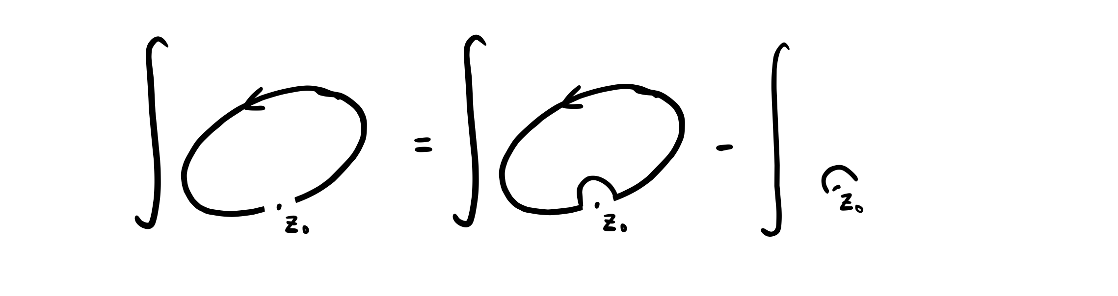
We add an indent around \( z_0 \) then subtract whatever that would have contributed to the integral. So what does the bump contribute?

where \( \theta_0 \) is whatever angle \( f(z) \) makes with the horizontal at \( z_0 \). If \( z_0 \) is a simple pole, then we have a series expansion of \( f(z) \)

\[f(z_0 + \epsilon e^{i \theta}) i \epsilon e^{i \theta} = i a_{-1} + i \sum_{n=0} ^\infty a_n (\epsilon e^{i \theta})^n\] \[\rightarrow _{\epsilon \rightarrow 0} i a_{-1}\]

So the principal value is equal to the indented contour integral, plus half the residue of the singularity along the path.

With this, we can write down a modified residue theorem for the principle value integral:

\[\]

Modified Residue Theorem

If \( f(z) \) has poles inside and on \( C \), then

\[P \oint_C f(z) \dd z = 2 \pi i \sum \text{Res}(f(z); z_0 \text{ inside } C) + \pi i \sum \text{Res}(f(z); z_0 \text{ on } C)\]

This is only possible if the poles on \( C \) are simple poles, otherwise the bump contour integral goes to infinity.

These improper integrals also come up in inverse Laplace transforms, but generally they appear there if we have missed some physical constraint such as causality (e.g. the function you’re transforming is assumed to be 0 for all time before \( t = 0 \), in order for the transform to be valid).) Improper integrals can also appear in physics PDEs if we ignore viscosity. But we’ll find if we put even a little bit of viscosity back in, the singularity moves just off the contour and we see that everything is actually fine.

Example

Here, this is a proper integral (\( \lim_{x \rightarrow 0} f(x) = t \) ). But we want to use Jordan’s lemma to calculate the integral, closing it in the upper half plane. But we can’t close it because \( \sin(tx) \) blows up along the imaginary axis.

Since the original integral is proper, the principal value is the same as the regular value

There is a wrong way to do this:

Because the real component of \( e^{itx}/x \) has a singularity at \( x = 0 \). The real part is what turns it into an improper integral!

Instead, we start with the principal value:

Here we’ve introduced an improper integral \( \int_{-\infty}^{\infty}\frac{\cos(tx)}{x} \dd x \)

Now we can go back to using Jordan’s lemma to compute the result. Since \( |\frac{1}{z}| \rightarrow 0 \) as \( z \rightarrow \infty \), we can close the contour. We close it in the upper half plane if \( t > 0 \), or in the lower half plane if \( t < 0 \).

We use the modified residue theorem for this one. There are no singularities inside the contour, and the residue at \( z_0 = 0 \) is 1, so

For \( t < 0 \) the contour goes clockwise, so we add a negative sign

This gives us a pretty good step function:

What about \( t = 0 \)?

Another example:

Note the series expansion of cosine

\[\cos(ax) = 1 - \frac{(ax)^2}{2!} + \ldots\] \[\cos(bx) = 1 - \frac{(bx)^2}{2!} + \ldots\]

So the leading terms cancel and this is actually a proper integral

Use residue theorem, to get the residue multiply by \( x \) and take the limit as \( x \rightarrow 0 \)