Now we’re getting to the good stuff that would usually be skipped in undergraduate courses!
Consider the example
\[I = \int _{0} ^{\infty} \frac{x^{\alpha - 1}}{x + 1} \dd x \qquad 0 < \alpha < 1\]Previously, we’ve said we should refuse to compute the integral of a multi-valued function. But for a real value this integral is legit and well-defined.
First, observe that the integrand is a single-valued function. Numerically, you can just take the area under the curve and work out the result. But in the complex plane, we don’t know how to do it. The complex function
\[f(z) = \frac{z^{\alpha - 1}}{z + 1}\]is a multi-valued function. Now, the multi-valuedness that’s been introduced is our own fault, so we need to deal with it by defining a single-valued integrand by restricting the argument. How you restrict the argument will give you different functions as a result, but you should compute the same integral!
We pick \( 0 < \theta < 2 \pi \). We find that the function is discontinuous at the branch across \( 0 \leq x \leq \infty \) (\( A \neq B \) )
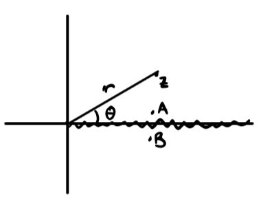
\[A: \quad \theta = 0 \qquad f(A) = \frac{(r e^{i 0})^{\alpha - 1}}{r e^{i 0} + 1} = \frac{r ^{\alpha - 1}}{r + 1}\] \[B: \quad \theta = 2 \pi \quad f(B) = \frac{(r e^{i 2 \pi})^{\alpha - 1}}{r e^{2 \pi i} + 1} = \frac{r^{\alpha - 1} e^{ 2 \pi i(\alpha - 1)}}{r + 1} = e^{ 2 \pi \alpha i} f(A)\]
If we cut the domain this way, we want to follow the contour along the real axis, then close the contour. We have to avoid the branch cut where the functino is not analytic, so we end up with this pac-man shaped contour.
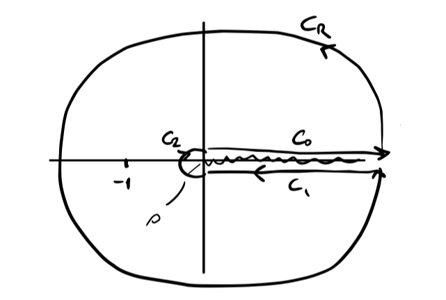
\( C_0 \) is what we want. \( C_R \rightarrow 0 \) and \( C_2 \rightarrow 0 \). Normally \( C_1 \) would cancel with \( C_0 \). In this case, one will be a multiple of the other, so we can still compute it.
Let’s convince ourselves that \( I = \int C_0 \)
\[\int _{C_0} = \int_{\rho} ^{R + \rho} \frac{(r e^{i 0^+})^{\alpha - 1}}{r e^{i 0^+} + 1} \dd (r e^{i 0^+}) \\ \lim_{\rho \rightarrow 0} \lim_{R \rightarrow \infty} = \int_{0} ^{\infty} \frac{x^{\alpha - 1}}{x + 1} \dd x = I\] \[\int_{C_1} = \int_R ^\rho \frac{(r e^{i 2 \pi^-})^{\alpha - 1}}{r e^{i 2 \pi ^-} + 1} \dd (r e^{i 2 \pi ^-}) \\ \lim_{\rho \rightarrow 0} \lim_{R \rightarrow \infty} = - e^{2 \pi \alpha i} \int_{0} ^{\infty} \frac{x^{\alpha - 1}}{x + 1} \dd x = - e^{ 2 \pi \alpha i} I\]But before we get ahead of ourselves, let’s waiti to take the \( \lim_{\rho \rightarrow 0} \) until we deal with \( z = 0 \) on \( C_2 \)
\[z = \rho e^{i \theta}\] \[\rho \rightarrow 0^+ \qquad \theta \text{ from } 2 \pi \text{ to } 0\]
\[\int_{C_2} f(z) \dd z = \int_{2 \pi} ^0 \frac{ \rho ^{\alpha - 1} e^{i (\alpha - 1) \theta}}{\rho e^{i \theta} + 1} e^{i \theta} \rho \dd \theta \\ \lim_{\rho \rightarrow 0} = \int_{2 \pi} ^0 \frac{ \rho^{\alpha - 1} e^{i (\alpha - 1) \theta}}{1} e^{i \theta} \rho \dd \theta \\ \rightarrow \int_{2 \pi} ^0 \rho ^\alpha e^{i \alpha \theta} \dd \theta \\ = \rho^\alpha \int_{2 \pi} ^0 e^{i \alpha \theta} \dd \theta \\ = \rho^\alpha \left. \frac{i e^{\alpha \theta}}{i \alpha}\right|_{2 \pi} ^{\theta = 0}\\ = 0\]On the big circle \( C_R \), \( \int_{C_R} f(z) \dd z \rightarrow 0 \text{ as } R \rightarrow \infty \) if \( |z f(z) | \rightarrow 0 \) as \( R \rightarrow \infty \)
\[\left| z \frac{z^{\alpha - 1}}{z + 1} \right| = \left| \frac{z^\alpha}{z + 1} \right| \leq \frac{|z^\alpha|}{|z| - 1} \\ \rightarrow |z| ^{\alpha - 1} \rightarrow 0 \text{ as } R \rightarrow \infty\]Putting all the pieces together,
\[\oint _C = \int_{C_0} + \int_{C_1} + \int_{C_2} + \int_{C_R} \\ = I - e^{2 \pi \alpha i} I \\ = 2\pi i \sum \text{Res} [ f(z) \text{ inside } C]\] \[\text{Res}[z =-1] = \lim_{z \rightarrow -1} \frac{(z + 1)z^{\alpha - 1}}{z + 1} \\ = \lim_{z \rightarrow e^{i \pi}} z^{\alpha - 1} = e^{i \pi (\alpha - 1)}\]\[I (1 - e^{2 \pi \alpha i}) = 2 \pi i e^{i \pi (\alpha - 1)}\] \[I = \frac{2 \pi i e^{(\alpha - 1) \pi i}}{1 - e^{2 \pi \alpha i}} = \frac{\pi}{\sin(\alpha \pi)}\]
Now we know how to do the general case \( \int_0 ^\infty x^{\alpha - 1} f(x) \dd x \)!
For example,
\[I = \int _0 ^{\infty} \frac{x^{\alpha - 1}}{x^2 + 1} \dd x \\ = \frac{- \pi e^{-\pi \alpha i}}{\sin (\alpha \pi)} \sum \text{Res} \frac{z^{\alpha - 1}}{z ^2 + 1} \text{ at } e^{\pi i / 2}, e^{3 \pi i / 2} \\ = \frac{\pi}{\sin \alpha \pi} \sin \left( \frac{1}{2}(\alpha + 1) \pi \right)\]In general, when trying to compute real integrals in the complex plane, we increase in difficulty as we further restrict the bounds of integration:
\[I = \int_{-\infty}^{\infty}f(x) \dd x\] \[\rightarrow I = \int _0 ^{\infty} f(x) \dd x\] \[\rightarrow I = \int _a ^b\]
Let’s take a look at how we might compute the second-hardest case, using \( \ln(z) \) as an assistant:
Complex Integrals with \( \ln (z) \)#
Often, a multi-valued integrand involving \( ln(z) \) is introduced to solve a related real integral. Consider:
\[I = \int_0 ^\infty \frac{\dd x}{1 + x^3} \dd x\]We’ve evaluated this in the past by closing the contour along the radial path \( \theta = 2 \pi / 3 \). But this doesn’t work in general for integrals of the form
\[I = \int _0 ^\infty f(x) \dd x\]There may not be any radial line that closes the contour in an analytic single-valued way. So instead, we try evaluating the integral of \( \ln (z) f(z) \)
\[J = \oint _C \ln (z) f(z) \dd z\]To make this single-valued, we restrict \( 0 \leq \text{arg}(z) < 2 \pi \). \( C \) is the closed “Pac-man” contour \( C_R + C_0 + C_1 + C_2 \) from the previous section:
Suppose \( f(z) \) is such that
\[| \int _{C_R} \ln (z) f(z) \dd z | \rightarrow 0 \qquad |z| \rightarrow \infty\]This si true provided \( |z^{1+\epsilon} f(z) | \rightarrow 0 \) for any \( \epsilon > 0 \). This is because \( |\ln(z)| \) is bounded by \( |z^\epsilon| \).
We also suppose that
\[|\int _{C_2} \ln(z) f(z) \dd z | \rightarrow 0 \quad \text{ as } |z| = \rho \rightarrow 0^+\]This is true if \( f(z) \) is bounded as \( |z| \rightarrow 0 \) because
\[\int _{C_2} \ln (z) f(z) = \int _{2 \pi} ^0 (\ln \rho + i \theta) \rho e^{i \theta} i f(\rho e^{i \theta}) \dd \theta\]and this would vanish as \( f(\rho e^{i \theta}) \rho \ln (\rho) \) when \( \rho \rightarrow 0 \).
On \( C_0 \): \( z = r e^{i 0} = r \)
\[\int _{C_0} = \int _0 ^\infty \ln(r) f(r) \dd r\]On \( C_1 \): \( z = r e^{2 \pi i} \)
\[\int _{C_1} = \int _{\infty} ^0 (\ln (r) + 2 \pi i) f(r e^{2 \pi i}) \dd r \\ = - \int _0 ^\infty \ln(r) f(r) \dd r - 2 \pi i \int _0 ^\infty f(r) \dd r\] \[\int _{C_0} + \int _{C_1} = \int _0 ^\infty \ln (r) f(r) \dd r - \int _0 ^\infty \ln (r) f(r) \dd r - 2 \pi i \int _0 ^{\infty} f(r) \dd r \\ = - 2 \pi i I\]
Putting it all together,
\[I = - \frac{1}{2 \pi i} \oint _C \ln (z) f(z) \dd z \\ = - \sum_{z_j} \text{Res} [ \ln (z) f(z); z_j]\]where \( 0 \leq \text{arg}(z) < 2 \pi \) and \( z_j \) are the poles of \( f(z) \), excluding the origin and positive real axis. For our example:
\[f(z) = \frac{1}{1 + z^3}\]On \( C_R \) : \( z = R e^{i \theta} \)
\[\int _{C_R} = \int _0 ^{2 \pi} \frac{(\ln R + i \theta)}{1 + R^3 e^{3 i \theta}}\] \[| \int _{C_R} | \leq \int _0 ^{2 \pi } \frac{R |\ln R + i \theta|}{|1 - R^3|} \dd \theta \rightarrow 0 \text{ as } R^{-2} \ln R \text{ as } R \rightarrow \infty\]
\[I = - \sum \text{Res} \frac{\ln (z)}{1 + z^3} \text{ at } e^{\pi i / 3}, e^{\pi i}, e^{5 \pi i / 3} \\ = - \frac{\ln e^{\pi i / 3}}{3 e^{2 \pi i / 3}} - \frac{\ln e^{\pi i}}{3 e^{2 \pi i}} - \frac{\ln e^{5 \pi i / 3}}{3 e^{10 \pi i / 3}} \\ = - \frac{\pi i}{9 e^{2 \pi i / 3}} - \frac{\pi i }{3} - \frac{5 \pi i }{9 e^{10 \pi i / 3}} \\ = \pi \frac{4}{9} \sin (\pi / 3) \\ = \frac{2 \pi}{3 \sqrt{3}}\]Let’s have another example:
\[I = \int _0 ^{\infty} \frac{\dd x}{x^2 + 3x + 2}\]This is a case where there’s no way to close the contour with a single-valued function, since there is no radial line other than \( \theta = 0, 2 \pi \ldots \) for which \( z^2 + 2 z + 2 \) is a constant multiple of \( r^2 + 3r + 2 \). But computing the related integral
\[\oint _C \frac{\ln (z) \dd z}{z^2 + 3z + 2}\]leads us to
\[I = - \sum \text{Res} \frac{\ln(z)}{z^2 + 3z + 2} = - \frac{\ln (e^{\pi i})}{-1} - \frac{\ln (2 e^{\pi i})}{1} = \ln (2)\]To generalize this:
Computing one-sided improper integrals with \( \ln (z) \)
\[I = \int _0 ^\infty f(x) \dd x = - \sum_{z_j} \text{Res}[ f(z) \ln (z); z_j]\]where \( 0 \leq \text{arg}(z) < 2 \pi \) and \( z_j \) are the poles of \( f(z) \) which do not lie on the positive real axis or the origin, and
\[|z^{1 + \epsilon} f(z) | \rightarrow 0 \text{ as } R \rightarrow \infty, \epsilon > 0\]
Suppose \( f(x) \) itself contains a \( \ln(x) \):
\[I = \int _0 ^{\infty} \frac{\ln(x)}{x^2 + a^2} \dd x \qquad a > 0\]Let \( f(x) = \ln (x) g(x) \) where \( g(x) = 1/x^2 + a^2 \) which is analytic. As before,
\[J = \oint _C \ln(z) f(z) \dd z = \oint _C (\ln (z))^2 g(z) \dd z\]Again, \( |\int _{C_R}| \rightarrow 0 \) and \( |\int _{C_2} | \rightarrow 0 \)
On \( C_0 \), \( z = r e^{i 0} = r \)
\[\int_{C_0} = \int _0 ^\infty (\ln r)^2 g(r) \dd r\]On \( C_1 \) , \( z = r e^{2 \pi i} \)
\[\int _{C_1} = \int _{\infty} ^0 (\ln (r) + 2 \pi i)^2 g(r) \dd r \\ = - \int _0 ^\infty (\ln (r))^2 g(r) \dd r - 4 \pi i \int _0 ^\infty \ln (r) g(r) \dd r + 4 \pi ^2 \int _0 ^\infty g(r) \dd r\] \[\int _{C_0} + \int _{C_1} = - 4 \pi i \int _0 ^\infty \ln (r) g(r) \dd r + 4 \pi ^2 \int _0 ^\infty g(r) \dd r \\ = - 4 \pi I + 4 \pi ^2 \int _0 ^\infty g(r) \dd r\] \[J = \oint _C = 2 \pi i \sum \text{Res} [ (\ln z)^2 g(z) ; z_j \text{ in } C]\] \[I = - \frac{1}{2} \sum \text{Res} [ (\ln z)^2 g(z)] - i \pi \int _0 ^\infty g(r) \dd r\] \[\int _0 ^\infty g(r) \dd r = - \sum \text{Res} [ \ln z g(z) ]\]Finite Integrals#
Now we get to the really hard stuff:
\[\int _a ^b f(x) \dd x\]For example, say we need to compute the real integral
\[I = \int _{-1} ^1 \left( \frac{1 - x}{1 + x} \right)^{1/3} \dd x\]Consider \( f(z) = \left( \frac{z - 1}{z + 1} \right)^{1/3} \). To make this multi-valued function single-valued, we need to place branch cuts and determine where the resulting function is continuous:
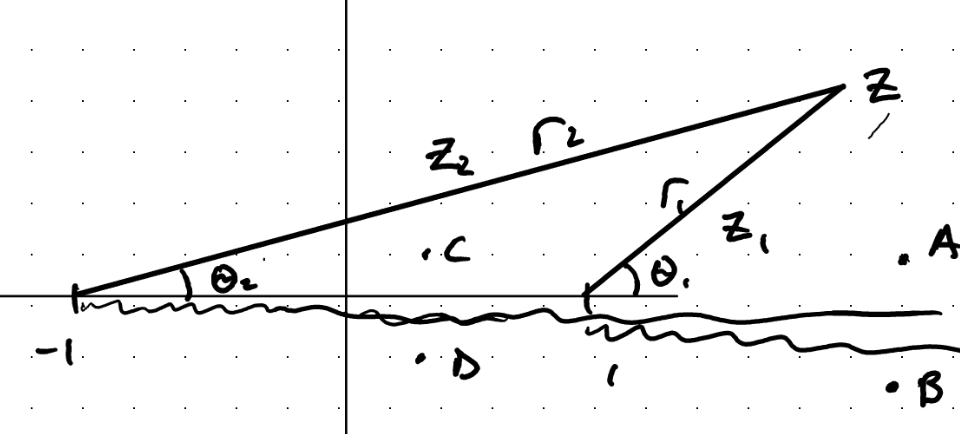
\[z - 1 = r_1 e^{i \theta_1} \qquad 0 \leq \theta_1 < 2 \pi\] \[z + 1 = r_2 e^{i \theta_2} \qquad - \leq \theta_2 < 2 \pi\]
\[A: \theta_1 = 0 \qquad \theta_2 = 0\] \[B: \theta_1 = 2 \pi \qquad \theta_2 = 2 \pi\]
So \( f(A) = f(B) \) and the function is continuous from \( 1 \rightarrow \infty \).
\[C: \theta_1 = \pi \qquad \theta_2 = 0\] \[D: \theta_1 = \pi \qquad \theta_2 = 2 \pi\] \[f(C) = \left( \frac{r_1}{r_2} \right)^{1/3} e^{i \pi / 3}\\ f(D) = \left( \frac{r_1}{r_2} \right)^{1/3} e^{-i \pi / 3}\]
So \( f(C) \neq f(D) \) and the branch cut remains between \( -1 \) and \( 1 \). We can close this contour with a “dumbell” contour
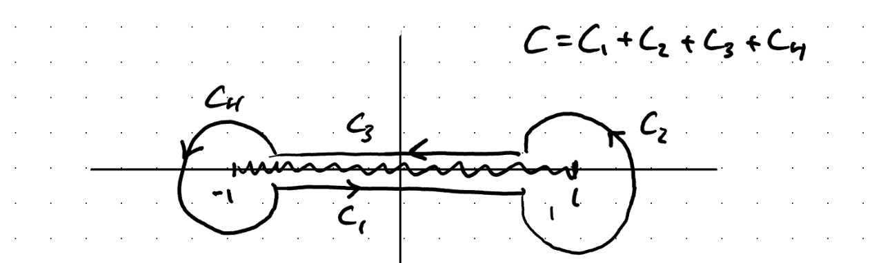
On \( C_1 \) :
\[x - 1 = z - 1 = r_1 e^{i \theta_1} \qquad \theta_1 = \pi \qquad r_1 = 1 - x\] \[x + 1 = z + 1 = r_2 e^{i \theta_2} \qquad \theta_2 = 2 \pi \qquad r_2 = 1 + x\]
\[\int_{C_1} f(z) \dd x = \int_{-1}^{1} \left( \frac{r_1}{r_2} \right) ^{1/3} e^{i (\theta_1 - \theta_2) / 3} \dd x \\ = \int_{-1} ^1 \left( \frac{1 - x}{1 + x} \right) ^{1/3} e^{- i \pi / 3} \dd x\]On \( C_3 \):
\[x - 1 = z - 1 = r_1 e^{i \theta_1} \qquad \theta_1 = \pi \qquad r_1 = 1 - x\] \[x + 1 = z + 1 = r_2 e^{i \theta_2} \qquad \theta_2 = 0 \qquad r_2 = 1 + x\] \[\int_{C_{3}} f(z) \dd z = \int _{-1} ^1 \left( \frac{r_1}{r_2} \right) ^{1/3} e^{i (\theta_1 - \theta_2) / 3} \dd x \\ = \int_{-1} ^{1} \left( \frac{1 - x}{1 + x} \right) ^{1/3} e^{i \pi / 3} \dd x\]
On \( C_2 \):
\[z - 1 = r_1 e^{i 0} \qquad r_1 \rightarrow 0\] \[\int_{C_2} \rightarrow 0 \text{ as } r_1 ^{1/3} r_1\]
On \( C_4 \):
\[\frac{1}{z + 1} = \frac{1}{r_2 e^{i \theta_2}}, \qquad r_2 \rightarrow 0\] \[\int _{C_4} \rightarrow 0 \text{ as } r_2 ^{-1/3} r_2\]
So the closed contour integral over \( C_1 + C_2 + C_3 + C_4 \) gives us a constant times the integral we want to do, so that’s good! But we can’t use the residue theorem because we’ve got a whole branch cut inside the contour!
\[\oint_C f(z) \dd z = (e^{- i \pi / 3} - e^{i \pi / 3} ) I\]One method we have is to deform the contour out to infinity
\[|z| = R \text{ on } C_R\]For large \( R \) we can expand \( f(z) \) in inverse powers of \( z \)
\[f(z) = \left( \frac{1 - \frac{1}{z}}{1 + \frac{1}{z}} \right)^{1/3}\]Using the binomial expansion,
\[\frac{1}{(1 + \frac{1}{z})^{1/3}} = (1 + \frac{1}{z})^{-1/3} \approx 1 - \frac{1}{3} \frac{1}{z} + \ldots\] \[f(z) \approx 1 - \frac{2}{3} \frac{1}{z} + ( ) z^2 + \ldots\]Then we compute the integral directly
\[\int_{C_R} f(z) \dd z = \int _0 ^{2 \pi} \left( 1 - \frac{2}{3} \frac{1}{R e^{i \theta}} + \ldots \right) R e^{i \theta} \dd \theta\]All terms except the first go to zero for large \( R \) and we’re left with
\[= - \frac{2}{3} 2 \pi i\] \[- \frac{4 \pi i}{3} = - 2 i \sin \frac{\pi}{3} I \quad \rightarrow \quad I = \frac{2 \pi}{3 \sin (\pi / 3)}\]Or, we could take method 2: flip the direction of \( C \) around so that it encloses points on the outside, in a negative sense. There, the only singularity is the point as \( \infty \), defined as
\[z = \frac{1}{t} \quad \text{ as } t \rightarrow 0\]\[\oint _C f(z) \dd z = - \oint _{C_{\infty}}f(z) \dd z\] So what is the residue of the point at infinity?
\[z = \frac{1}{t} \qquad \dd z = - \frac{1}{t^2} \dd t\] \[- \oint _{C_{\infty}} - \frac{1}{t^2} f(\frac{1}{t}) \dd t = \oint _{C_\infty} \frac{1}{t^2} f(\frac{1}{t}) \dd t = 2 \pi i \text{Res} (f(\frac{1}{t}); t = 0)\] \[f(t) = 1 + \frac{2}{3} t + ( ) t^2 + \ldots\] \[\frac{1}{t^2} f(\frac{1}{t}) = \frac{1}{t^2} - \frac{2}{3} \frac{1}{t} + \ldots\]So we can just pick out the residue as \( \text{Res(t = 0)} = - \frac{2}{3} \).
The most difficult case of all is the finite integral of a function which is analytic everywhere on the interval.
\[I = \int _a ^b f(x) \dd x\]Consider
\[g(z) = \ln \left[ \frac{(z - b)}{(z - a)} \right] f(z)\]and again, look at the dumbell contour in the z plane. The resulting function is of course multi-valued, so we need to restrict the arguments \[z_1 = r_1 e^{i \theta_1} \qquad z_2 = r_2 e^{i \theta_2}\] \[0 \leq \theta_1 < 2 \pi \qquad 0 \leq \theta_2 < 2 \pi\]
We check the continuity using the same A/B test as before
At \( A \):
\[\theta_1 = 0 \qquad \theta_2 = 0\] \[\ln \frac{z - b}{z - a} = \ln \frac{ r_1 e^{i \theta_1}}{r_2 e^{i \theta_2}} = \ln \frac{r_1}{r_2} + i (\theta_1 - \theta_2)\]
At \( B \):
\[\theta_1 = 2 \pi \qquad \theta_2 = 2 \pi\]So \( g(A) = g(B) \) and the function is continuous from \( b \rightarrow \infty \)
At \( C \):
\[\theta_1 = \pi \qquad \theta_2 = 0\] At \( D \): \[\theta_1 = \pi \qquad \theta_2 = 2 \pi\]
Since \( g(C) \neq g(D) \) the branch cut remains between \( a \rightarrow b \). Now we try to compute the integral over the dumbell contour \( C \)
\[J = \oint _C \ln \frac{z - b}{z - a} \dd z\]Along the bottom,
\[z = x - i \epsilon \qquad \theta_1 = \pi \qquad \theta_2 = 2 \pi\] \[g(z) = \left[ \ln \frac{b - x}{x - a} - i \pi \right] f(z)\]
Along the top,
\[z = x + i \epsilon \qquad \theta_1 = \pi \qquad \theta_2 = 0\] \[g(z) = \left[\ln \frac{b - x}{x - a} + i \pi \right] f(z)\]On the little circles:
\[z = b + \epsilon e^{i \theta} \qquad \dd z = \epsilon e^{i \theta} \dd \theta\] \[g \sim \ln \epsilon f(b) \qquad g \dd z \sin \epsilon \ln \epsilon f(b) \rightarrow 0 \text{ as } \epsilon \rightarrow 0\]
So now we’ve just got the two straight segments. But we want \( \int f(z) \), not \( \int \ln \frac{b - z}{a - z} f(z) \). Lucky for us, some things are about to cancel nicely:
\[\oint _C g(z) \dd z = \int _a ^b f(z) \left( \left[ \ln \frac{b - x}{x - a} - i \pi \right] - \left[ \ln \frac{b - x}{x - a} + i \pi \right] \right) \dd x \\ = - 2 \pi i \int _a ^b f(x) \dd x\] \[I = \int _a ^b f(x) \dd x = - \frac{1}{2 \pi i} \oint _C g(z) \dd z\]We could almost have anticipated this result from the beginning, because the discontinuity in \( g(z) \) is only in the argument, not the imaginary part. So we’ve successfully enclosed a contour. But we’ve enclosed a branch cut in doing so, so the residue theorem does not apply. So as usual with the dumbell contour, we can add a minus sign and find the residues of \( g(z) \) outside of \( C \), plus the residue at infinity
\[\oint_C g(z) \dd z = - 2 \pi i \sum \text{Res} ( f(z) ; z_j \text{ outside } C) + 2 \pi i \sum \text{Res} ( \frac{1}{t^2} f(\frac{1}{t}); t \rightarrow 0)\] \[I = \int _a ^b f(x) \dd x = \sum \text{Res}[ g(z) ; z_j \text{ in the cut plane }] - \text{Res} [ \frac{1}{t^2} f(\frac{1}{t}); t \rightarrow 0]\](Just as a note on the sign flipping here, we have \( -2 \pi i \sum \text{Res} \) because we flipped the contour inside out. We get another sign flip for the residue at infinity from \( \dd z \rightarrow - \frac{1}{t^2} \dd t \) )