Fourier Transform #

It’s good to start out with the definition of a Fourier transform:

[]

Fourier Transform

\[\mathcal{F}(f(t)) \equiv F(\lambda) \equiv \int_{-\infty}^{\infty}e^{i \lambda t} f(t) \dd t\]

Note: \( t \) does not necessarily denote time, as it generally does in the Laplace transform. It’s just a dummy variable in the integration and is often a spatial coordinate.

To recover \( f(t) \) we also have the inverse Fourier transform

\[f(t) = \mathcal{F} ^{-1} (F(\lambda)) = \frac{1}{2 \pi} \int_{-\infty}^{\infty}e^{- i \lambda t} F(\lambda) \dd \lambda\]

\[\]

Fourier’s Theorem

This is what gives us the ability to write down the inverse transform. We won’t derive the theorem here since that is usually done in an earlier course. The general approach starts with the Fourier series expansion and takes the limit to converge to the Riemann sum of the integral. The theorem states:

\[f(t) = \frac{1}{2 \pi} \int_{-\infty}^{\infty} \dd \lambda \int_{-\infty}^{\infty}\dd \tau e^{i \lambda ( \tau - t)} f(\tau)\]

This is valid for any piecewise smooth \( f(t) \) which is integrable.

If we think about it, it’s amazing that we can recover \( f(t) \) after all of that. The key is that \( e^{i \lambda t}, e^{-i \lambda t} \) form a complete, orthogonal basis for all piecewise smooth integrable functions.

For consistency, we need to make sure we consistently place the \( \pm \) exponent on the transform and the factor of \( 1/2 \pi \), since they are arbitrary choices.

“Piecewise smooth” means that over any interval, we can subdivide into a finite number of pieces where the function is smooth. We can have a finite number of jumps, but the function can never jump to infinity.

Example:

As a real integral, this isn’t the easiest thing to do. But we can use Jordan’s lemma to make it simple for us. \( 1 / z^2 + 4 \) gotes to zero as \( |z| \rightarrow \infty \), so

Let’s take our inverse transform for a spin to show that it works!

This is pretty cool, but in real life the powerful use of the transform is in solving partial differential equations.

Fourier Transform of Derivatives #

We’ve required that \( f(t) \) is integrable, so the boundary term must vanish. \( f(t) |^{\pm \infty} = 0 \). This is actually a pretty major restriction on Fourier transforms. Many familiar functions are not totally integrable, but we often want to use their Fourier transform. The generalized Fourier transform solves this by restricting the transform in the direction that is integrable, then setting the function to zero in the other direction. This is very related to the Laplace transform, which is always one-sided.

Let’s do some examples

\[f(t) = e^{- t} \quad \rightarrow \quad F(\lambda) = \int_{-\infty}^{\infty}e^{i \lambda t - t} \dd t = \left.\frac{1}{i \lambda - 1} e^{i (\lambda - 1)t} \right|_{-\infty} ^{\infty}\] This limit does not exist as \( t \rightarrow -\infty \). Similarly, the transform of \( f(t) = e^{t} \) blows up as \( t \rightarrow \infty \). To overcome this we, can consider a one-sided version of the function

These functions do have a well-defined Fourier transform

\[f(t) = \begin{cases} e^{-i \lambda_0 t} & t \geq 0 \\ 0 & t < 0 \end{cases}\] \[F(\lambda) = \int _0 ^\infty e^{i (\lambda - \lambda _0)t} \dd t = \frac{e^{i (\lambda - \lambda_0)t}}{i (\lambda - \lambda_0)}\]

This limit does not exist for purely real \( \lambda \), since it oscillates forever in the \( + \infty \) direction. But if there is a small positive imaginary part of \( \lambda \) then the limit is \[F(\lambda) = \frac{i}{\lambda - \lambda_0}\]

Now we want an inverse Fourier transform for this:

Now we’ve made ourselves an improper integral. But at least we know how we got here! (it was by letting \( \text{Im}(\lambda) > 0 \) ). We should not try to convert this into a principal value integral, because we will get a different answer that way.

Instead, we need to modify the inverse transform! This is because Fourier’s theorem is only valid for an integrable function. So how should we fix it? If \( f(t) \) is not integrable, but \( g(t) = e^{- \alpha t} f(t) \) is integrable (e.g. \( f(t) \sim e^{a t} \rightarrow g(t) \sim e^{-(\alpha - a)t} \) if \( \alpha > a \) ). The Fourier theorem then applies to \( g(t) \)

So, we can relate \( G(\lambda) \) to \( F(\lambda + i \alpha) \). We know the inverse transform for \( G(\lambda) \)

\[g(t) = \frac{1}{2 \pi } \int_{-\infty}^{\infty}e^{- i \lambda t} G(\lambda) \dd \lambda \\ = \frac{1}{2 \pi} \int_{-\infty}^{\infty}e^{- i \lambda t} F( \lambda + i \alpha) \dd \lambda\] \[f(t) = \frac{1}{2 \pi} \int_{-\infty}^{\infty}e^{-i (\lambda + i \alpha) t} F(\lambda + i \alpha) \dd \lambda\] (let \( \hat{\lambda} = \lambda + i \alpha \) ) \[f(t) = \frac{1}{2 \pi} \int_{-\infty + i \alpha}^{\infty + i \alpha} e^{- i \hat{\lambda} t} F(\hat{\lambda}) \dd \hat{\lambda}\]

For our example, we just need \( \alpha > 0 \) to make \( g(t) \) integrable. Now the contour of integration sits just above the real axis.

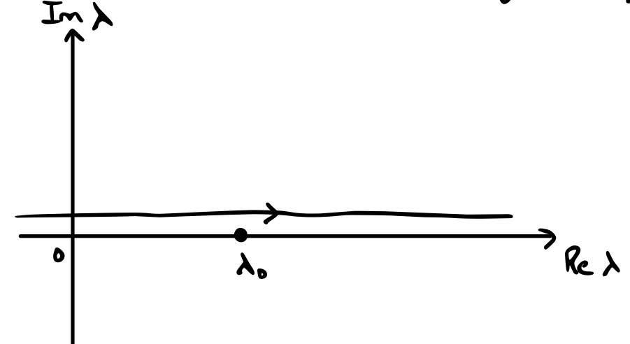
By Cauchy’s theorem, this is the same as the indented contour going just above \( \lambda_0 \)

We can use Jordan’s lemma for this. For \( t < 0 \), \( e^{- i \lambda t} \) has a positive exponent so we close in the upper half plane. Closing above, we now have a contour that does not contain any singularities, so \( f(t) = 0 \). That’s exactly what we think we should get for our single-sided function.

For \( t > 0 \), we need to close in the lower half plane, so we enclose the singularity at \( \lambda = \lambda_0 \)

and we’ve successfully recovered our one-sided \( f(t) \).

In general, if we go from \( f(t) \) to \( F(\lambda) \) and we find that \( f(t) \) is not integrable, then \( F(\lambda) \) exists for some \( \text{Im}(\lambda) > \alpha \)

is not singular on the real axis, and the inverse transform should integrate along \( (- \infty + i \alpha, \infty + i \alpha) \) i.e. above the axis.

Of course, in most applications we don’t have prior knowledge of \( f(t) \). We usually end up with a partial differential equation where we have assumed an expression for \( F(\lambda) \). Given the \( F(\lambda) = i / (\lambda - \lambda_0) \), this appears to give an improper integral

In this case, we should not just take the principal value integral because integrating along the contour is not the same as the principal value limit! The correct approach is to apply the causality condition! If we end up with a singularity on the path of integration, then something must be wrong with the physics of the problem. Taking the indented contour going just above the singularity corresponds with allowing for a small \( \text{Im}(\lambda) > 0 \), which means \( f(t) \) does not diverge faster than \( e^{\alpha \lambda} \) for some \( \lambda > 0 \).

Laplace Transform #

We all know \( \mathcal{L} \) from our undergrad differential equations or electronics classes, but we never got the inverse transform back then, so let’s fill in that gap.

The Laplace transform is the same as the one-sided Fourier transform with \( -i \lambda \) replaced by \( s \) (or \( -s = + i \lambda \) )

This makes a couple of things clearer. The Laplace transform integral that looked like a completely real integrand actually has a purely imaginary argument in the exponential. And when we look at the inverse Fourier transform, with \( -s = i \lambda \), the integral is actually going up and down in the imaginary direction

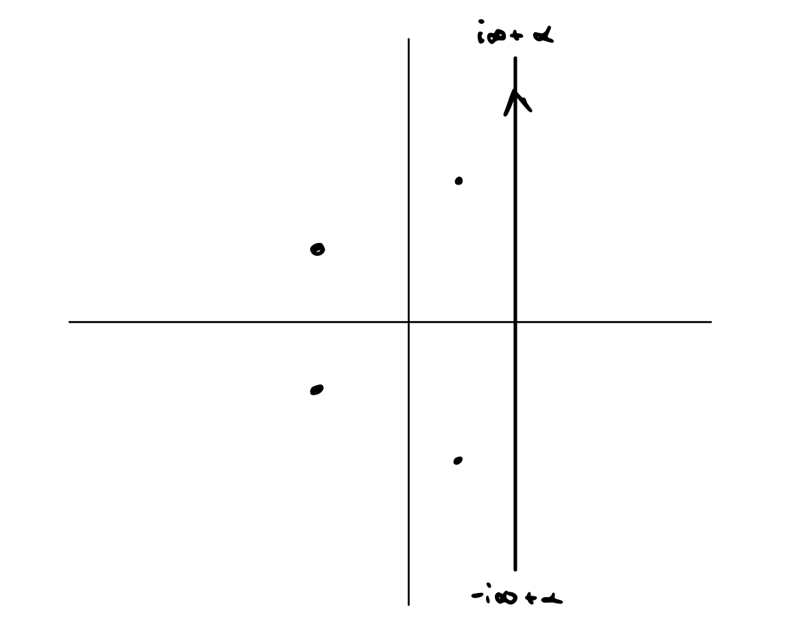
The path we take to close the contour depends on the sign of \( t \). For \( t < 0 \), we close on the right by Jordan’s lemma (just rotate everything by \( \pi / 2 \) ). As it turns out, to make the function integrable, we must take \( \alpha \) to be to the right of all singularities of \( f(t) \). Since that is the case, there are no poles to the right of the contour and we get zero.

Closing to the left,

in the complex plane if there are no branch cuts or branch points. If you do have a branch cut in \( f(s) \), then we modify the Bromwich contour like this:

Example:

\[\mathcal{L} [1] = \int _0 ^{\infty} e^{-st} \dd t = \frac{e^{-st}}{s} |_{0} ^{\infty} = \frac{1}{s} \quad \text{ if } \text{Re}(s) > 0\] \[\mathcal{L}^{-1} [\frac{1}{s}] = \frac{1}{2 \pi i} \int_L e^{st}{s} \dd s = \begin{cases} \text{Res} [\frac{e^{st}}{s}; s = 0] & t > 0 \\ 0 & t < 0 \end{cases} \\ = \begin{cases} 1 & t > 0 \\ 0 & t < 0 \end{cases}\]

Laplace Transform of Derivatives #

\[\mathcal{L} [f'(t)] = \int _0 ^{\infty} e^{-st} f'(t) \dd t \\ = e^{-st} f(t) |_0 ^{\infty} + s \int _0 ^\infty e^{-st} f(t) \dd t \\ = s \mathcal{L} [f(t)] - f(0)\] \[\mathcal{L} [f''(t)] = s \mathcal{L} [f(t)] - f(0) - f'(0)\]

where we assume that \( e^{-st} f(t) \rightarrow 0 \) and \( e^{-st} f’(t) \rightarrow 0 \) as \( t \rightarrow \infty \).

We want to use Laplace transforms to solve differential equations. In particular, the spicy partial differential equations. Let’s start with the wave equation:

\[\pdv{^2}{t^2} u - c^2 \pdv{^2}{x^2} u = 0 \qquad -\infty < x < \infty \qquad t > 0\] with boundary conditions

\[u \rightarrow 0 \quad \text{ as } x \rightarrow \pm \infty\] \[u(x, 0) = f(x) \qquad \pdv{}{t} u(x, 0) = 0 \qquad (\text{or } g(x))\] First, define \( U(\lambda, t) \) as the Fourier transform of \( u \) in \( x \)

Here, we are starting to play fast and loose with the rules, and we will make the pure mathematicians mad :) We should prove that a solution \( u(x, t) \) to our PDE actually exists, and that the solution is integrable (so its Fourier transform exists). But it’s way easier to ask for forgiveness than to ask for permission. We assume both of these. If we find \( u(x, t) \), then it exists and we can check for integrability after the fact.

We aren’t given \( \pdv{}{x} u \rightarrow 0 \) as \( x \rightarrow \pm \infty \), but we’ll assume it to get rid of the boundary terms. There’s another thing we need to come back and check at the end!

\[\mathcal{F}\left[ \pdv{^2u}{x^2} \right] = - \lambda^2 U\] \[\mathcal{F} \left[ \pdv{^2 u}{t^2} \right] = \pdv{^2}{t^2} \mathcal{F}[u]\]

So the wave equation now looks like \[\pdv{^2}{t^2} U = - (c \lambda)^2 U\] \[\rightarrow U(\lambda, t) = A(\lambda) \cos (c \lambda t) + B(\lambda) \sin (c \lambda t)\]

Applying boundary conditions,

\[\pdv{}{t} U(\lambda, 0) = 0 \qquad U(\lambda, 0) = F(\lambda) = \mathcal{F}[f(x)]\] \[\rightarrow B(\lambda) = 0 \qquad A(\lambda) = F(\lambda)\] \[U(\lambda, t) = F(\lambda) \cos (c \lambda t)\] \[u(x, t) = \mathcal{F}^{-1} [U(\lambda, t)] = \frac{1}{2 \pi} \int_{-\infty}^{\infty}U(\lambda, t) e^{- i \lambda t} \dd \lambda\\ = \frac{1}{2 \pi } \int_{-\infty}^{\infty}F(\lambda) \cos (c \lambda t) e^{- i \lambda t} \dd \lambda \\ = \frac{1}{2 \pi} \int_{-\infty}^{\infty}\frac{1}{2} F(\lambda) e^{- i \lambda (x - ct)} \dd \lambda + \frac{1}{2 \pi} \int_{-\infty}^{\infty}\frac{1}{2} F(\lambda) e^{- i \lambda( x + ct)} \dd \lambda\]

But by definition,

so

So, are we done? No! We took some shortcuts that we still need to justify. If \( f(x) \) is of compact support, then we’re good on the \( f(x \rightarrow \pm \infty) \) and \( f’(x \rightarrow \pm \infty) \) boundary conditions. Also as long as \( f(x) \) has a Fourier transform, then \( u(x, t) \) also has a Fourier transform. That means our bases are covered and we have nothing to apologize for.

Solving the Heat Equation #

The heat equation is a nice application for these transforms to solve PDE’s:

\[\pdv{u}{t} - \alpha \pdv{^2 u}{x^2} = 0\] \[- \infty < x < \infty \qquad t > 0 \qquad \alpha > 0\]

This problem is ill-posed if we try to solve for \( t < 0 \) (imagine trying to solve the diffusuion equation to find the initial distribution of what eventually becomes a uniform distribution everywhere) and \( \alpha < 0 \) (for the same reason).

The boundary conditions for the problem are:

\[u \rightarrow 0 \text{ as } x \rightarrow \pm \infty\] \[u(x, 0) = g(x)\]

We don’t know if \( u \) is integrable, but let’s assume the Fourier transform exists and come back to check later once we’ve solved \int_{-\infty}^{\infty}

Note: at this point we could have approached this problem in a number of ways. We could take the Fourier transform of \( u(x, t) \) in \( x \), or we could take the Laplace transform of \( u(x, t) \) in \( t \), or we could take the one-sided Fourier transform in \( t \), or we could take the Laplace transform in \( x \). But doing the Fourier transform in \( x \) is the right choice here, because we’re starting with a homogeneous equation and we have infinite boundary conditions in \( x \). This means that once we’ve taken the transform, we should not end up with any boundary terms and we’ll be left with a homogeneous equation. Since the PDE is only first-order in \( t \), that means we’ll be left with a first-order homogeneous ODE, and that’s very easy for us to solve.

\[\mathcal{F} [ \pdv{u}{t} ] = \pdv{}{t} U\] \[\mathcal{F}[\pdv{^2 u}{x^2} ] = \int_{-\infty}^{\infty}e^{i \lambda x} \pdv{^2 u}{x^2} \dd x \\ = e^{i \lambda x} \pdv{u}{x} |_{-\infty} ^{\infty} - i \lambda \int_{-\infty}^{\infty}e^{i \lambda x} \pdv{u}{x} \dd x \\ = e^{i \lambda x} \pdv{u}{x} |_{-\infty} ^{\infty} - i \lambda u e^{i \lambda x} |_{-\infty} ^{\infty} + (i \lambda) ^2 U\]

Again, we assume that \( \pdv{u}{x} \rightarrow 0 \) as \( x \rightarrow \pm \infty \) to get rid of the boundary terms. And again, we’ll have to come back and verify this once we’re done

Applying our initial conditions,

\[U(\lambda, 0) = A(\lambda) = G(\lambda) = \mathcal{F}[g(x)]\] \[U(\lambda, t) = \mathcal{F}[g(x)] e^{- \alpha \lambda ^2 t}\] \[u(x, t) = \frac{1}{2 \pi} \int_{-\infty}^{\infty}e^{-i \lambda x} G(\lambda) e^{- \alpha \lambda ^2 t} \dd \lambda\]

We can go further here using the convolution properties of \( \mathcal{F} \), but for now let’s apply what we have to some examples

\[g(x) = \delta (x) \qquad (\text{Dirac delta function})\] \[\mathcal{F}[g(x)] = \int_{-\infty}^{\infty}e^{i \lambda x} g(x) \dd x = \int_{-\infty}^{\infty}e^{i \lambda x} \delta(x) \dd x = e^{i \lambda (0)} = 1\] \[u(x, t) = \frac{1}{2 \pi} \int_{-\infty}^{\infty}e^{-i \lambda x} (1) e^{- \alpha \lambda^2 t} \dd \lambda\]

We solve this by completing the square in the exponent to get a Gaussian integral of the form \( \int e^{- a x^2} = \sqrt{\pi / a} \). The general formula we’ll use for this is:

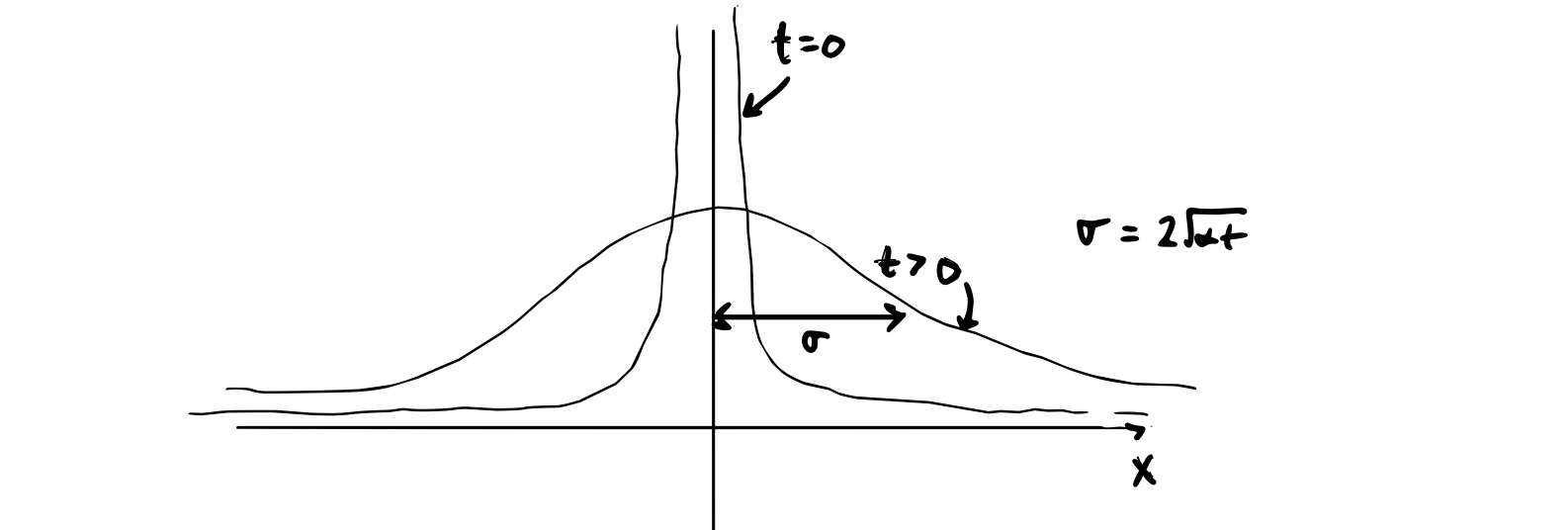
Now let’s consider the intermediate case where we start with a Gaussian

\[g(x) = B e^{- \beta x^2}\] Using the formula above, \[G(\lambda) = \sqrt{\frac{\pi}{\beta}} B e^{- \lambda ^2 / 4 \beta}\] The Fourier transform of a Gaussian is another Gaussian. If the original function was sharply peaked, then the transform is very flat, and vice versa.

For the \( \delta(x) \) initial condition, we took the easy way out by taking the Fourier transform in space to end up with a nice clean homogeneous 1st order ODE. Now let’s see what would happen if we do it the stupid way. This is an especially useful approach to go through because some problems don’t yield analytic solutions, so we should know a bit about how to apply asymptotic analysis to solve these kinds of problems with inverse Laplace transforms that introduce branch cuts.

\[\text{PDE}: \quad \pdv{u}{t} = \alpha \pdv{^2u}{x^2} \qquad - \infty < x < \infty \qquad t > 0\] \[\text{BC:} \quad u \rightarrow 0 \text{ as } x \rightarrow \pm \infty \qquad u(x, 0) = \delta(x)\]

Let’s take the Laplace transform in time:

If the real part of \( s \) is greater than zero, then this is integrable and

Good for us, now we’ve made a 2nd order non-homogeneous ODE. One approach is to take the Fourier transform, so that \( \delta(x) \) becomes \( 1 \), and then we need to take both inverse Fourier and Laplace transforms to get the solution. Here, instead we’ll use Green’s functions since \( \delta(x) = 0 \) if \( x \neq 0 \).

For \( x > 0 \) :

There’s that square root in the argument, whcih we got from our first-order terms, and that’s where we’ll get a branch cut.

In the \( +x \) direction we can apply \( u \rightarrow 0 \) as \( x \rightarrow \infty \)

otherwise, \( A = 0 \). Let’s choose \( C = 0 \). This seems like an arbitrary decision, but as long as we remain consistent we should get the right answer (modulo some annoying difficulties down the road).

For \( x < 0 \):

\[\pdv{^2 \hat{u}}{x^2} - \frac{s}{\alpha} \hat{u} = 0\] \[\hat{u}(x, s) = B e^{\sqrt{\frac{s}{\alpha}} x } + D e^{-\sqrt{\frac{s}{\alpha}} x }\]

Now we need to bring in \( u(0, x) \) using a matching condition. We’ll do this by integrating the ODE across \( x = 0 \):

\[\int _{0^-} ^{0^+} \left( \pdv{^2 \hat{u}}{x^2} - \frac{s}{\alpha} \hat{u} \right) \dd x = - \frac{1}{\alpha} \int _{0^-} ^{0^+} \delta (x) \dd x\] \[\pdv{}{x} \hat{u} |_{0^-} ^{0^+} - \frac{s}{\alpha} \int _{0^-} ^{0^+} \hat{u} \dd x = - \frac{1}{\alpha}\]

Here we need to make some arguments to determine the form of \( \hat{u} \). If \( \hat{u}(x = 0) \) is finite, then the integral over a vanishing interval is zero. On the other hand, if \( \hat{u} \) itself contains a delta function, then if we plug it back into the original differential equation we see that there is no way to match the singularity of \( \pdv{^2 u}{x^2} \) with the other finite terms. So \( \hat{u} \) must be finite at \( x = 0 \) and we end up with the jump condition

This is a finite jump condition, so \( \hat{u} \) must be continuous across the jump. Otherwise we would have a singularity on the left side that would need to match the constant on the right side.

so, at \( x = 0 \), for continuity we must have \( A = 0 \) and

\[\pdv{}{x} \hat{u} |_{0^+} = - A \sqrt{\frac{s}{\alpha}}\] \[\pdv{}{x} \hat{u} |_{0^-} = B \sqrt{\frac{s}{\alpha}}\] \[\left. \pdv{\hat{u}}{x} \right| _{0^-}^{0^+} = - \frac{1}{\alpha} \quad \rightarrow \quad A = \frac{1}{2 \sqrt{\alpha s}} = B\] \[\hat{u}(x, s) = \frac{1}{2 \sqrt{\alpha s}} e^{- \sqrt{\frac{s}{\alpha}} |x|}\]

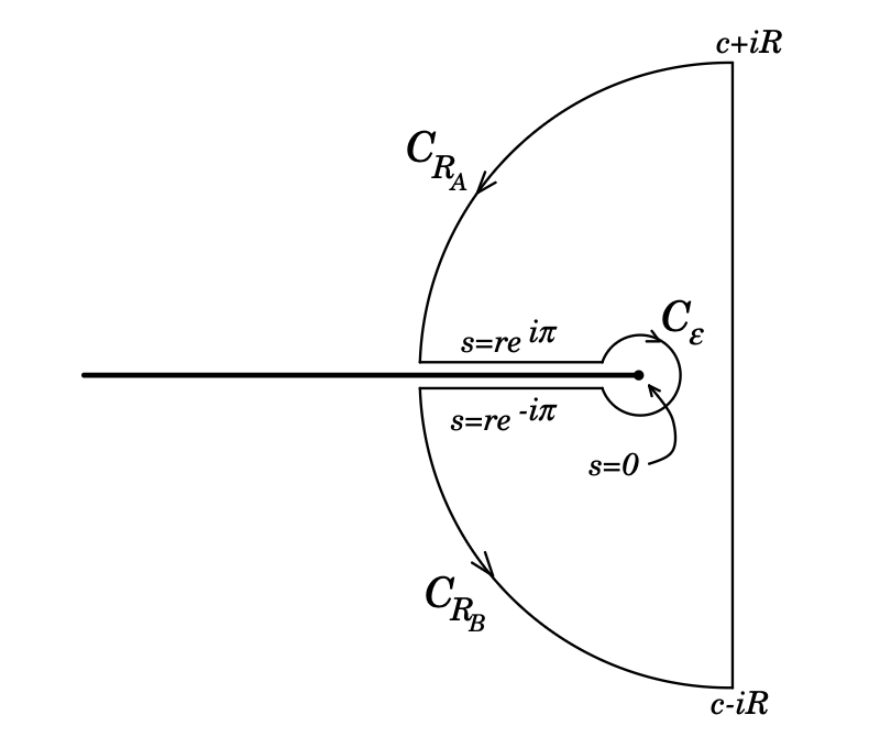
We still need to define a branch cut to make \( \hat{u} \) single-valued, otherwise we’ll have to refuse to integrate it.

Here, we need to make use of the fact that we require \( \text{Re}(s) > 0 \) for integrability, where

\[\text{Re} \sqrt{s} = r^{1/2} \cos (\theta / 2)\] \[\rightarrow \cos (\theta / 2) > 0 \qquad \rightarrow \qquad - \pi < \theta < \pi\]

Now we can attempt the inverse Laplace transform, but the contour we need to use is a bit complicated:

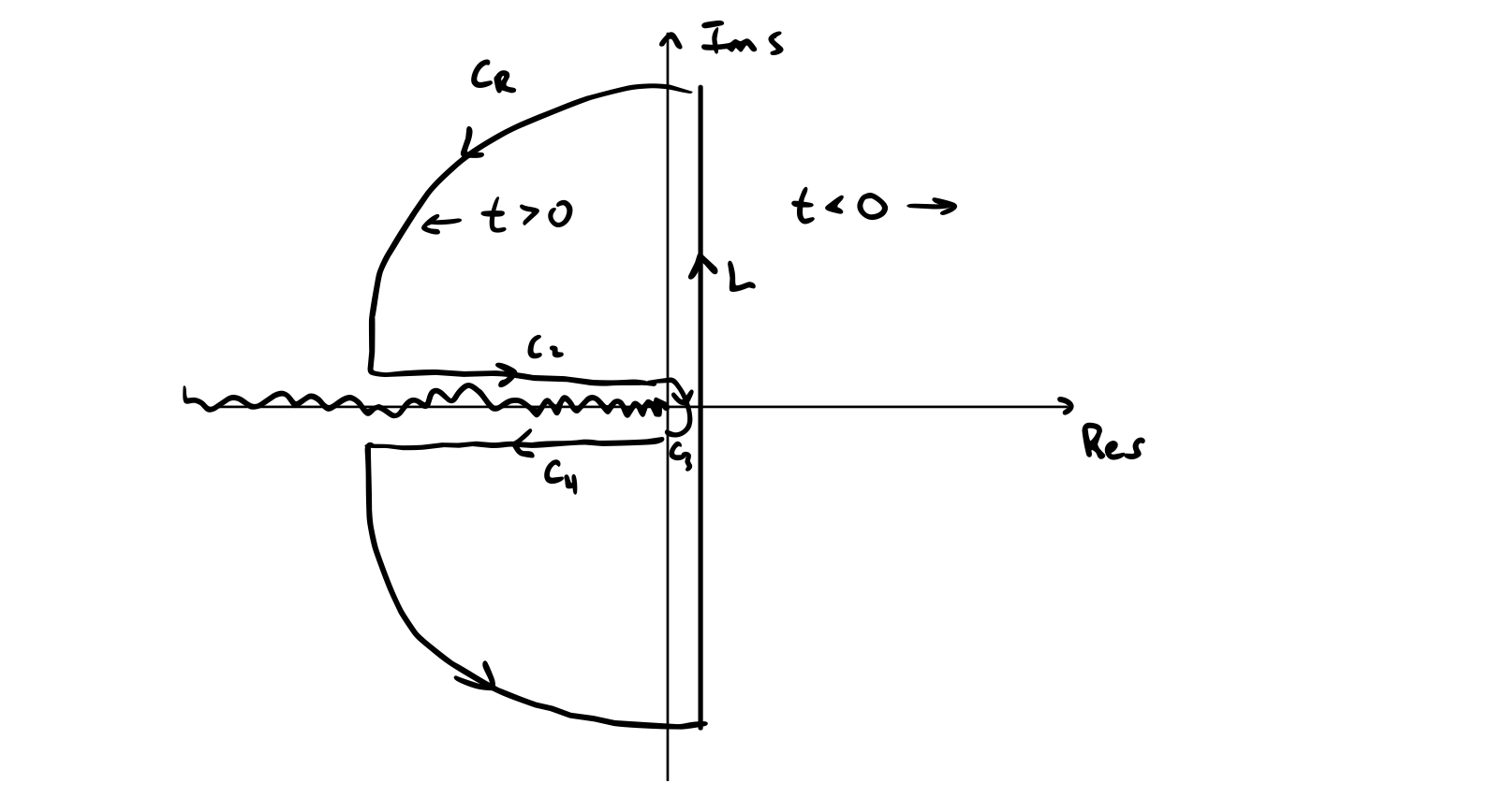
There are no singularities contained, so

On \( C_2 \):

\[s = r e^{i \theta} \qquad \theta = \pi ^-\] \[\sqrt{s} = r^{1/2} e^{i \pi / 2}\] \[\frac{1}{2 \pi i} \int _{C_2} = \frac{1}{2 \pi i} \int _{\infty} ^0 \frac{e^{-r6 - i \sqrt{\frac{r}{\alpha}}|x|} e^{i \pi}}{2 i \sqrt{\alpha r}} \dd r \\ = - \frac{1}{4 \pi \sqrt{\alpha}} \int_0 ^\infty e^{-rt - i \sqrt{\frac{r}{\alpha}}|x|} \dd r\]

So we end up with

Let \( y^2 = r \) so that \( 2y \dd y = \dd r \) (so that we can get rid of the square roots)

Then we can complete the square to get a normal Gaussian integral