Conformal Mappings #

There are many physical problems that require us to solve the Laplace equation on a domain \( D \) with some set of boundary conditions. As we’ve seen so far, there are certain sets of boundary conditions for which Laplace’s equation is relatively easy to solve: for instance a Dirichlet boundary condition on a circle, or in the upper half-plane. But most of the time we are given more complicated geometries for the domain and boundary that require trickier approaches. One way of solving these problems is to perform a specific type of change of variables to map the original complicated domain to a simpler one that we already know how to solve.

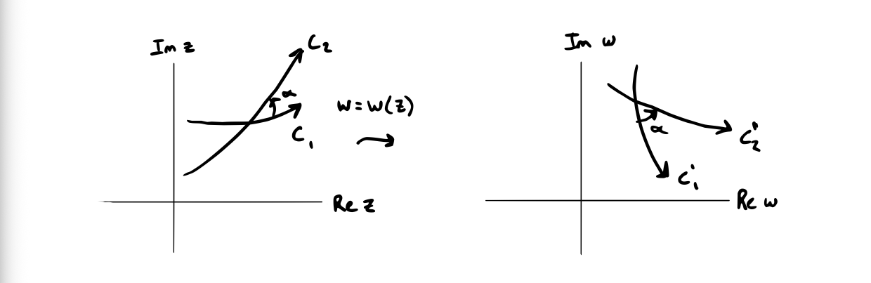
A conformal mapping is a mapping which preserves both the magnitude and sense of angles. The funny thing is when we work with conformal mappings to solve problems, we will mostly be looking for places where a mapping is not conformal. For the definition:

A mapping which preserves the magnitude and sense of the angle between two smooth arcs passing through a specific point is said to be conformal at that point.

[]

Theorem

At each point where \( w(z) \) is analytic and \( w’(z) \neq 0 \), the mapping \( w = w(z) \) is conformal.

We’ll come back to prove this later, but that isn’t the important part for us.

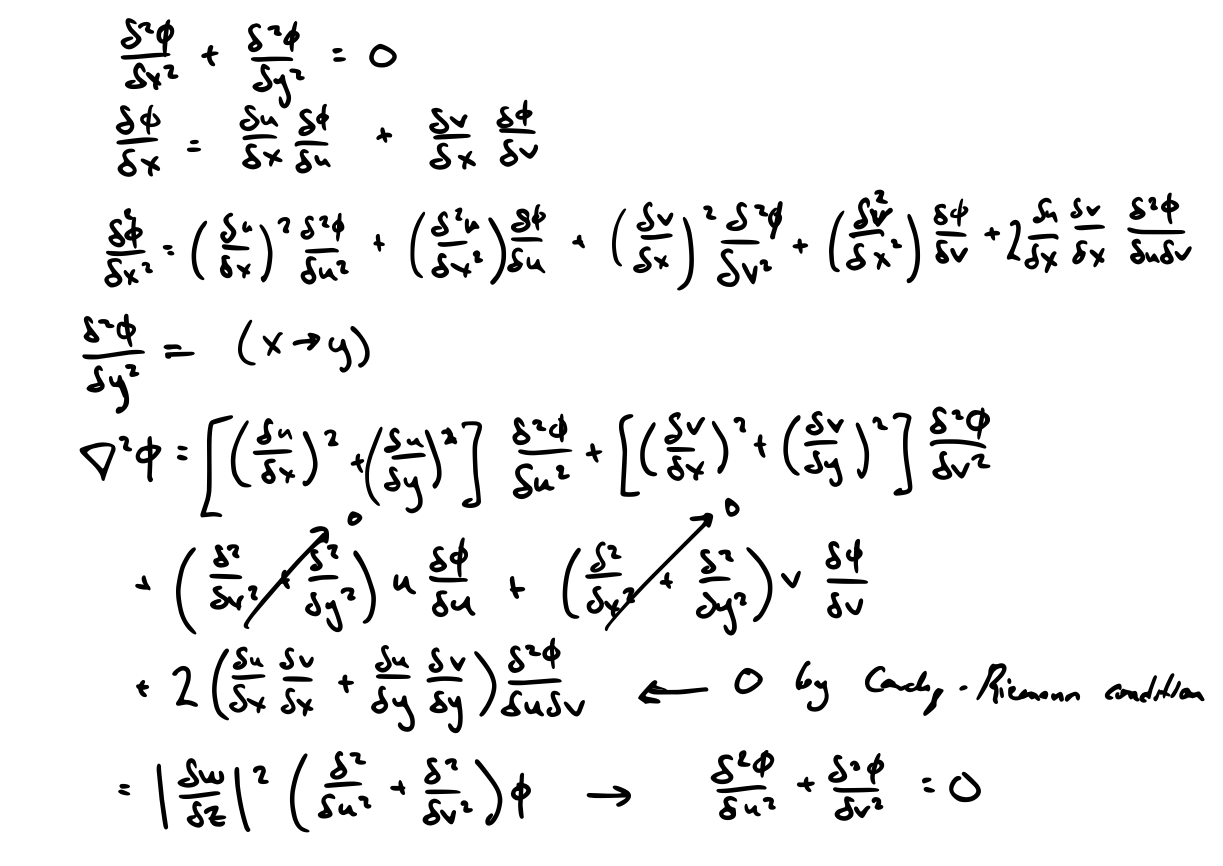
Let’s take a look at invariance of the Laplace equation under a conformal mapping

If \( w \) is conformal, then \( \nabla ^2 _w \phi = \pdv{^2 \phi}{u^2} + \pdv{^2 \phi}{v^2} = 0 \)

As we know, in numerical analysis we frequently use conformal mappings to solve problems in a simpler geometry than the physical geometry.

Showing the invariance of the Laplace equation under a conformal mapping is pretty easy, but it is tedious:

(can’t be bothered to type all that out again right now…)

The takeaway here is that Laplace’s equation is unaffected by a conformal mapping. So if \( \phi \) solves Laplace’s equation in the \( z \) plane, then its image in the \( w \) plane also satisfies Laplace’s equation.

How do we know what sort of mapping to use for our particular boundary conditions? The answer is basically people have made tables of conformal mappings that are useful for particular types of boundary conditions; just look in the back of a complex analysis textbook to find the one we need

Example:

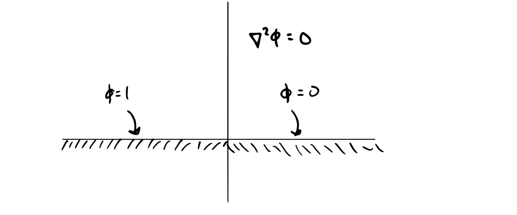
Consider the branch of \( \ln(z) \):

This function is analytic everywhere except \( z = 0 \) and along the positive real axis. So the function \[\psi = \text{Im} f(z) = \frac{1}{\pi} \theta\]

\( \psi \) should satisfy the Laplace equation in regions where \( f(z) \) is analytic.

The constants of \( \psi \) are like rays out from the origin - streamlines for a source flow. The particular problem that \( \psi \) solves looks like this:

Another example: electrostatic potential in a cylindrical conductor:

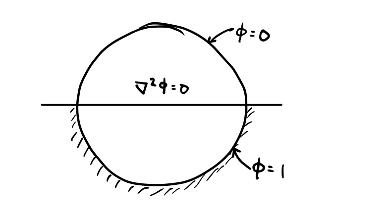
We want to convert the circle into a straight line, and the interior into the upper half plane. To transform circles into straight lines requires a bilinear transformation:

We pick \( z_0 = -1 \) to map point \( C \) to infinity. Then we map \( a \) to the origin by picking \( z_1 = 1 \). Then choose \( A = -i \) so the image lies flat

\[w(z) = i \frac{z - 1}{z + 1}\] \[\phi = \frac{1}{\pi} \ln w \\ = \frac{1}{\pi} \text{arg} w \\ = \frac{1}{\pi} \text{arg} \left( i \frac{z - 1}{z + 1} \right) \\ = \frac{1}{\pi} \tan^{-1} \left( \frac{1 - x^2 - y^2}{2y} \right) \quad 0 \leq \theta < 2 \pi\]

In the \( w \) plane, the unit circle is

This is real, so \( v = 0 \). The interior of the circle is the upper half plane \( v > 0 \).

Types of Transformations #

Translation #

The origin in the \( z \) plane is just shifted to \( c \) in the \( w \) plane

Rotation #

\[w = w(z) = e^{i \phi} z\] \[\text{arg} w = \phi + \text{arg} z\]

this is just a rotation through the angle \( \phi \)

Magnification #

\( \rho > 1 \) is a magnification, \( \rho < 1 \) is a reduction.

Linear transformation #

Write \( a = \rho e^{i \phi} \)

\[w_1 = e^{i \phi} z \qquad \text{(rotation)}\] \[w_2 = \rho w_1 \qquad \text{(magnification)}\] \[w = w_2 + b \qquad \text{(translation)}\]

Inversion #

(i) The unit circle in the \( z \) plane is mapped to the unit circle in the \( w \) plane. But the inside of the unit circle is mapped to the outside and vice versa. The origin is mapped into infinity (as we’d expect since the transformation is not analytic at \( z = 0 \))

(ii) A circle which does not pass through \( z = 0 \) is mapped into a circle that does not pass through \( w = 0 \)

\[(x - x_0)^2 + (y - y_0) ^2 = R^2 \qquad (R^2 \neq x_0 ^2 + y_0 ^2)\] \[(\frac{u}{u^2 + v^2}) ^2 + (- \frac{v}{u^2 + v^2} - y_0 )^2 = R^2\] \[u^2 + v^2 + \frac{2 x_0 u - 2 y_0 v - 1}{R^2 - (x_0 ^2 + y_0 ^2)} = 0\] \[( u + \frac{x_0}{R^2 - (x_0 ^2 + y_0 ^2)})^2 + (v - \frac{y_0}{R^2 - (x_0 ^2 + y_0 ^2)})^2 = \frac{R^2}{[R^2 - (x_0 ^2 + y_0 ^2)]^2}\]

(iii) Straight lines passing through \( z = 0 \) are mapped into straight lines passing through \( w =0 \)

\[Ax - By = 0\] \[Au + Bv = 0\]

(iv) A straight line in the \( z \) plane not passing through the singularity \( z = 0 \) is mapped into a circle in the \( w \) plane passing through \( w = 0 \)

\[A \frac{u}{u^2 + v^2} + \frac{B v}{u^2 + v^2} = C\] \[u^2 + v^2 - \frac{A}{C} u - \frac{B}{C} v = 0\] \[(u - \frac{A}{2C})^2 + (v - \frac{B}{2C})^2 = (\frac{A}{2C})^2 + (\frac{B}{2C})^2\]

Conversely,

(v) A circle passing through \( z = 0 \) is mapped into a straight line in the \( w \) plane not passing through \( w = 0 \)

Shifted inversion #

Even more general, we can have

\( z = 0 \) previously becomes \( z = z_0 \), and \( w = 0 \) becomes \( w = w_0 \)

(i) The unit circle centered at \( z_0 \) in the \( z \) plane is mapped into a unit circle with center \( w_0 \)

(ii) A circle that does not pass through \( z = z_0 \) is mapped into a circle that does not pass through \( w = w_0 \)

(iii) Straight lines passing through \( z =z_0 \) are mapped into circles passing through \( w = w_0 \)

(iv) A straight line not passing through \( z = z_0 \) is mapped into a circle passing through \( w = w_0 \) . This is easier to understand if you look at the inverse: if I have a circle and a point passes through a singularity of the mapping, then the iamge must be infinite - a straight line.

(v) A circle passing through \( z =z_0 \) is mapped into a straight line not passing through \( w = w_0 \) (just the reciprocal of (iv))

Bilinear transformation #

Even more general, we come to the bilinear transformation

if \( A \) is real and positive, this magnifies the above case. If \( A \) is complex, then it magnifies and rotates. The extra degree of freedom afforded by \( A \) allows us to specify the orientation of the geometric shapes. It can also be written as

Many times, textbooks will write this as

but that is a bit misleading, because there are really only three degrees of freedom here (e.g. divide the top and bottom by \( d \) and the transform is the same).

The point \( z_0 \) indicates where a singularity exists in the \( z \) plane. The reverse is true for \( w_0 \) which indicates a singularity in the \( w \) plane.

Now let’s really dig into our previous example of finding the steady-state temperature distribution in a circular disk of unit radius where the temperature is prescribed to have two values on different portions of the circle. We used

The point \( z_0 = -1 \) is point \( c \) on the circle. By making that point correspond with the singularity in \( w \), that point is mapped to infinity. We can then pick some other point (\( a \)) in the \( z \) plane to lie on the straight line in the \( w \) plane. It is convenient to do this in our case because there is a jump condition in our problem along \( y = 0 \).

Looking at point \( b \),

And looking at point \( d \):

We can check the inside/outside mapping of the unit circle by picking a point inside the circle and checking where it gets mapped to. The origin is the easiest one:

That gets us in the upper half plane, so that’s where the interior of the circle gets mapped to.