ODEs, PDEs, and the Need for Numerical Methods#
In this class we focus on solution methods for ordinary differential equations (ODEs) and partial differential equations (PDEs). An ODE involves functions of a single variable and their derivatives, while a PDE involves functions of multiple variables and their partial derivatives.
ODEs#
A typical first-order ODE is
\[\dv{u}{t} = f(t, u)\]where \( u : [a, b] \to \mathbb{R} \) is the unknown and \( f : [a, b] \times \mathbb{R} \to \mathbb{R} \) is given. We call \( f \) the right-hand side (RHS) of the ODE, or a forcing term in a physical context. Higher-order ODEs often take the form
\[\frac{\dd^n u}{\dd t^n} = f\left(t, u, \dv{u}{t}, \frac{\dd^2 u}{\dd t^2}, \ldots, \frac{\dd^{n-1} u}{\dd t^{n-1}}\right)\]with \( f : [a, b] \times \mathbb{R}^n \to \mathbb{R} \). This is an \( n^{\text{th}} \)-order ODE. ODEs model anything whose evolution is described by its rate of change, which is why we usually think of \( u \) as a function of time \( t \).
Example: Harmonic Oscillator#
Ya boy the harmonic oscillator is the classic example
\[\frac{\dd^2 u}{\dd t^2} + \omega^2 u = 0 \qquad \omega = \sqrt{k/m}\]where \( u(t) \) is the displacement of a mass \( m \) from equilibrium, attached to a wall by a spring with constant \( k \).
Physically, the state of the system should depend on its condition at some initial time (take \( t = 0 \)). It is natural to specify the initial conditions (ICs): the initial displacement and velocity
\[u(0) = u_0 \qquad \dv{u}{t}(0) = v_0\]With these, the problem can be solved analytically
\[u(t) = u_0 \cos(\omega t) + \frac{v_0}{\omega} \sin(\omega t) \qquad \forall \, t \geq 0\]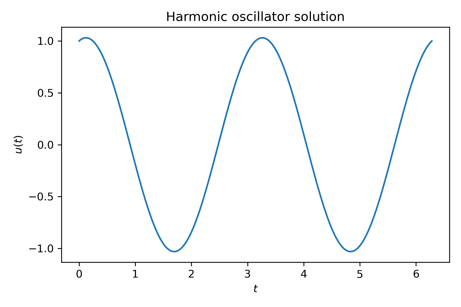
Analytic solution with \( u_0 = 1 \), \( v_0 = 0.5 \), \( \omega = 2 \).
Systems of ODEs#
ODE models extend naturally to several quantities that depend on each other, i.e. a system of interacting components. Replace the scalar \( u(t) \) with a vector-valued function
\[\vec{u} : [a, b] \to \mathbb{R}^d \qquad \vec{u}(t) = \left(u_1(t), \ldots, u_d(t)\right)\]so that
\[\frac{\dd^n \vec{u}}{\dd t^n} = \vec{f}\left(t, \vec{u}, \dv{\vec{u}}{t}, \ldots, \frac{\dd^{n-1} \vec{u}}{\dd t^{n-1}}\right) \qquad \vec{f} : [a, b] \times (\mathbb{R}^d)^n \to \mathbb{R}^d\]Example: Compartmental Disease Model#
Consider the spread of disease in a population, divided into compartments by disease status
\[\vec{u}(t) = \left(S(t), I(t), R(t)\right)\]\( S(t) \) susceptible, \( I(t) \) infected, \( R(t) \) recovered. Here \( n = 1 \) and the dynamics are
\[\dv{S}{t} = -\beta S I \qquad \dv{I}{t} = \beta S I - \gamma I \qquad \dv{R}{t} = \gamma I\]- \( \beta S I \) is the rate at which susceptible people are infected (infection rate \( \beta \))
- \( \gamma I \) is the rate at which infected people recover (recovery rate \( \gamma \))
This is the “SIR” model (Kermack & McKendrick, 1927). It’s overly simple: it assumes recovered people gain permanent immunity. Still, different choices of \( \beta, \gamma \) give qualitatively different dynamics: a fast and severe epidemic, a slow and mild one, or the disease dying out entirely. We need ICs for all three compartments; below uses \( S(0) = 0.95 \), \( I(0) = 0.05 \), \( R(0) = 0 \).
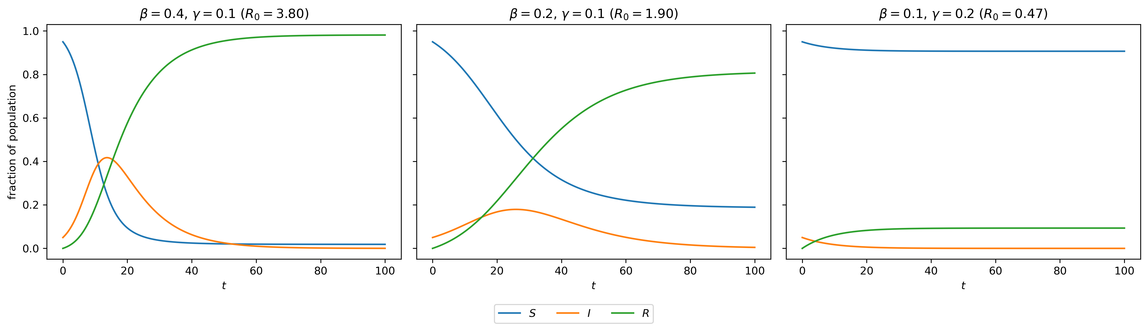
SIR dynamics from a forward Euler solver. Left: fast, severe epidemic. Center: slower, milder epidemic. Right: the disease dies out.
Unlike the harmonic oscillator, these solutions are numerical. Even simple-looking models hit a complexity wall where analytical methods fail, and we need numerical algorithms. This becomes even more apparent with PDEs.
PDEs#
A typical second-order PDE in space-time takes the form
\[\pdv{u}{t} = f\left(t, u, \pdv{u}{x}, \frac{\partial^2 u}{\partial x^2}\right)\]where now \( u : [0, T] \times [0, L] \to \mathbb{R} \) depends on both time and space, which makes this fundamentally different from the ODE setup.
Example: Heat Equation#
The heat (diffusion) equation describes the temperature \( u(t, x) \) in a 1D region over time
\[\pdv{u}{t} = \alpha \frac{\partial^2 u}{\partial x^2}\]where \( \alpha > 0 \) is the thermal diffusivity. To fully specify the problem we need boundary conditions, e.g. zero Dirichlet
\[u(t, 0) = u(t, L) = 0 \qquad t \geq 0\]and an initial condition
\[u(0, x) = u_0(x) \qquad x \in [0, L]\]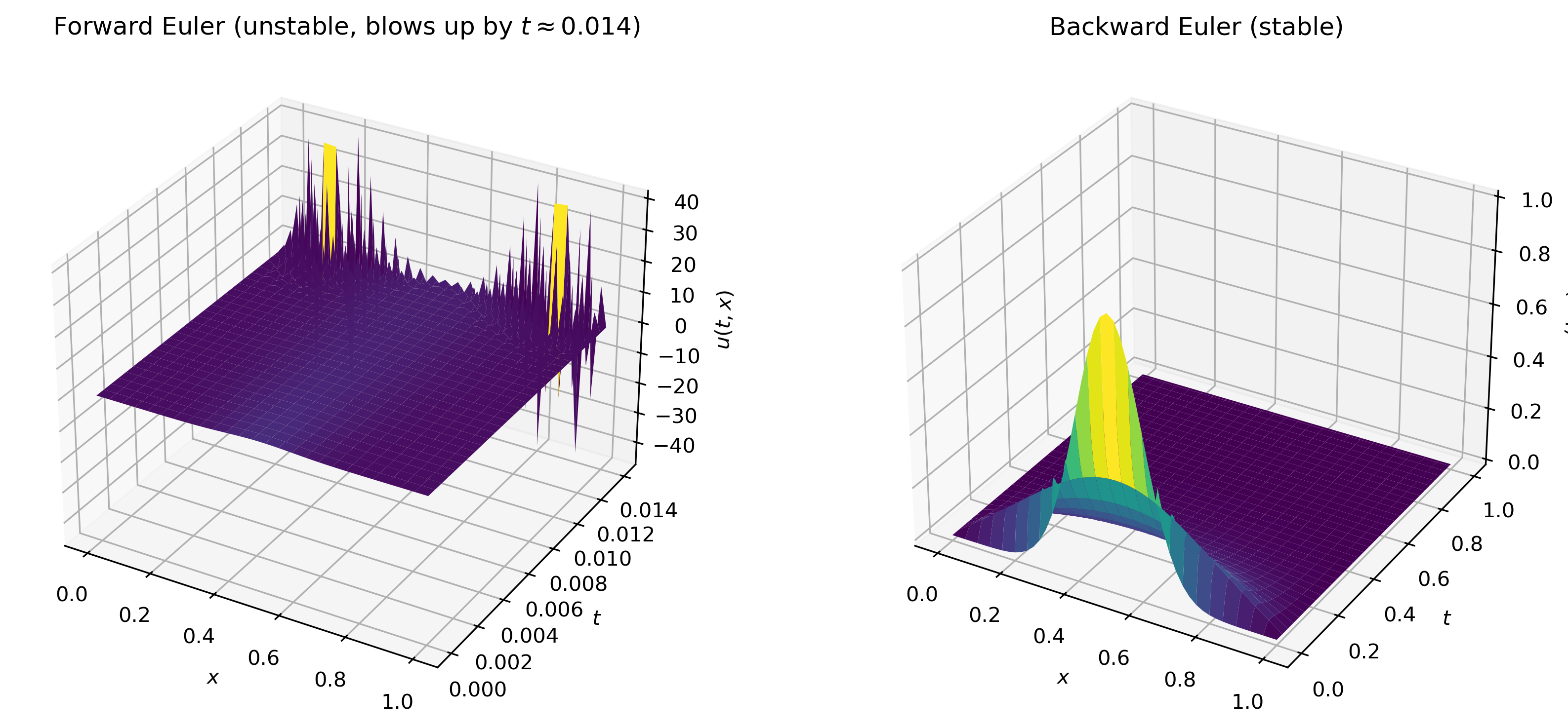
Left: an unstable numerical solution giving nonsense. Right: a stable numerical solution.
The left solution is clearly unphysical: heat should spread smoothly, not oscillate erratically. This is a numerical artifact, and understanding it (stability) is a major theme of the course.