Euler’s Methods for Solving IVPs#

We begin with the two simplest and most widely used methods, both named after Leonhard Euler: the forward and backward Euler methods. Throughout, consider a first-order IVP

where we want to estimate the solution on a finite interval \( [0, T] \). Everything here extends immediately to systems of ODEs, and hence to higher-order problems.

Well-Posedness#

Before approximating \( u(t) \) at all, we should ask whether the analytic problem is solvable in a reasonable sense. We adopt Hadamard’s notion: a problem is well-posed if

1. A solution exists
2. The solution is unique
3. The solution depends continuously on the data

For ODEs, this means existence and uniqueness of \( u(t) \), plus continuous dependence on the initial data: if we perturb \( u_0 \) slightly, the trajectory \( u(t) \) only changes slightly. People working on dynamical systems and ODEs give us a very useful theorem (see e.g. Perko, Differential Equations and Dynamical Systems, Sec. 2.2–2.3).

Theorem: Well-posedness of IVPs

Consider the IVP

\[\dv{\vec{u}}{t} = \vec{f}(t, \vec{u}) \qquad \vec{u}(0) = \vec{c}\]

Suppose \( \vec{f} : [0, T] \times \mathbb{R}^d \to \mathbb{R}^d \) is continuous in its domain and Lipschitz continuous in \( \vec{u} \), i.e. there exists \( L > 0 \) such that

\[\| \vec{f}(t, \vec{u}) - \vec{f}(t, \vec{v}) \| \leq L \| \vec{u} - \vec{v} \| \quad \forall \, (t, \vec{u}), (t, \vec{v}) \in [0, T] \times \mathbb{R}^d\]

Then:

1. (Existence and uniqueness) There exists a unique solution \( \vec{u}(t) \) for any \( \vec{c} \in \mathbb{R}^d \).
2. (Continuous dependence on initial data and RHS) Suppose \( \vec{r} : [0, T] \times \mathbb{R}^d \to \mathbb{R}^d \) is a bounded perturbation of \( \vec{f} \), i.e. there exists \( M > 0 \) such that \( \| \vec{r}(t, \vec{u}) \| \leq M \) for all \( (t, \vec{u}) \in [0, T] \times \mathbb{R}^d \). Further let \( \hat{\vec{u}}(t) \) be the solution to the perturbed problem

\[\dv{\hat{\vec{u}}}{t} = \vec{f}(t, \hat{\vec{u}}) + \vec{r}(t, \hat{\vec{u}}) \qquad \hat{\vec{u}}(0) = \hat{\vec{c}}\]

and assume such a solution exists and is unique. Then

\[\| \vec{u}(t) - \hat{\vec{u}}(t) \| \leq \underbrace{e^{Lt} \| \vec{c} - \hat{\vec{c}} \|}_{\text{perturbation of initial condition}} + \underbrace{\frac{M}{L} \left( e^{Lt} - 1 \right)}_{\text{perturbation due to } \vec{r} \text{ (modified system)}} \quad \forall \, t \in [0, T]\]

This is stronger than Hadamard’s notion: treating both the initial data and the RHS as “data”, we get not just continuous but Lipschitz continuous dependence on them. With peace of mind that the analytic problem is well-posed, we can go approximate it.

Euler’s Methods: An Application of Taylor’s Theorem#

Since IVPs describe the evolution of dynamic quantities, we approximate \( u(t) \) at a discrete set of times. Take \( [0, T] \) and partition it

We want to approximate the values \( u(t_n) \) with a set of quantities \( \{u_n\}_{n=0}^{N} \) , i.e. \( u_n \approx u(t_n) \) .

• The \( \{t_n\}_{n=0}^{N} \) are the discrete time points, or time mesh/grid points
• \( \Delta t_n \equiv t_{n+1} - t_n \) is the time step (or step size)
• The \( \{u_n\}_{n=0}^{N} \) are sometimes called the mesh function, but usually just the discrete solution
• If \( \Delta t_n = \Delta t \) is constant, we have a uniform mesh. Assume this from here on.

Forward (Explicit) Euler#

Taylor expand! Forward direction

Throw away the \( \mathcal{O}(\Delta t^2) \) error to get the explicit formula

This is the explicit Euler (forward Euler) method. We only need the current value \( u_n \) and the function \( f \): plug \( u_n \) into \( f \) to compute the next value. It truly embodies the intuition of “marching forward in time”. Rewritten in its more faithful form,

we see it’s based on a particular discretization of the time derivative. Other approximations of the derivative give other numerical methods — which raises the question of whether some are better than others.

Backward (Implicit) Euler#

Instead, Taylor expand about \( t_{n+1} \)

Again throw away the error term

Now \( u_{n+1} \) is only defined implicitly in terms of \( f(t_{n+1}, u_{n+1}) \) , so this is the implicit Euler (backward Euler) method. It seems only slightly different and less convenient: to compute \( u_{n+1} \) we have to solve a (possibly nonlinear) equation at each step. But there’s a profound difference between the two methods.

Comparing Forward and Backward Euler on the Test ODE#

Consider the “test ODE”

with exact solution \( u(t) = c e^{\lambda t} \). We allow complex \( \lambda \) because this becomes important when we deal with systems. Below, \( \lambda = -0.8 + 0.2i \), \( c = 1 \), on \( [0, 10] \).

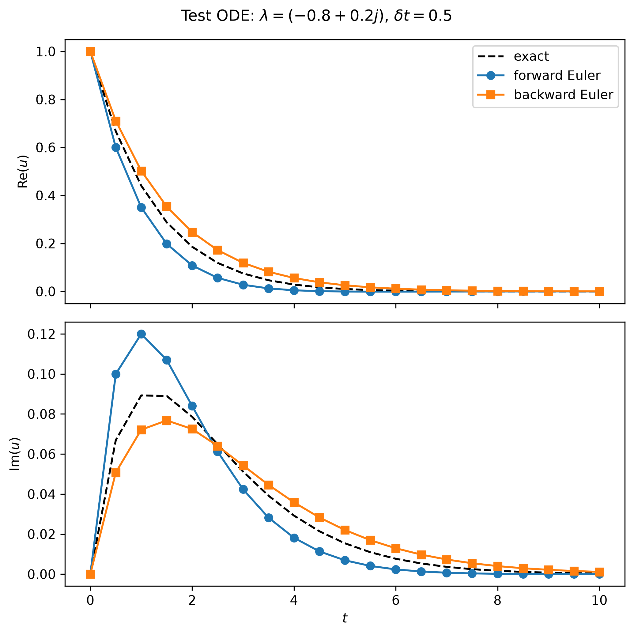
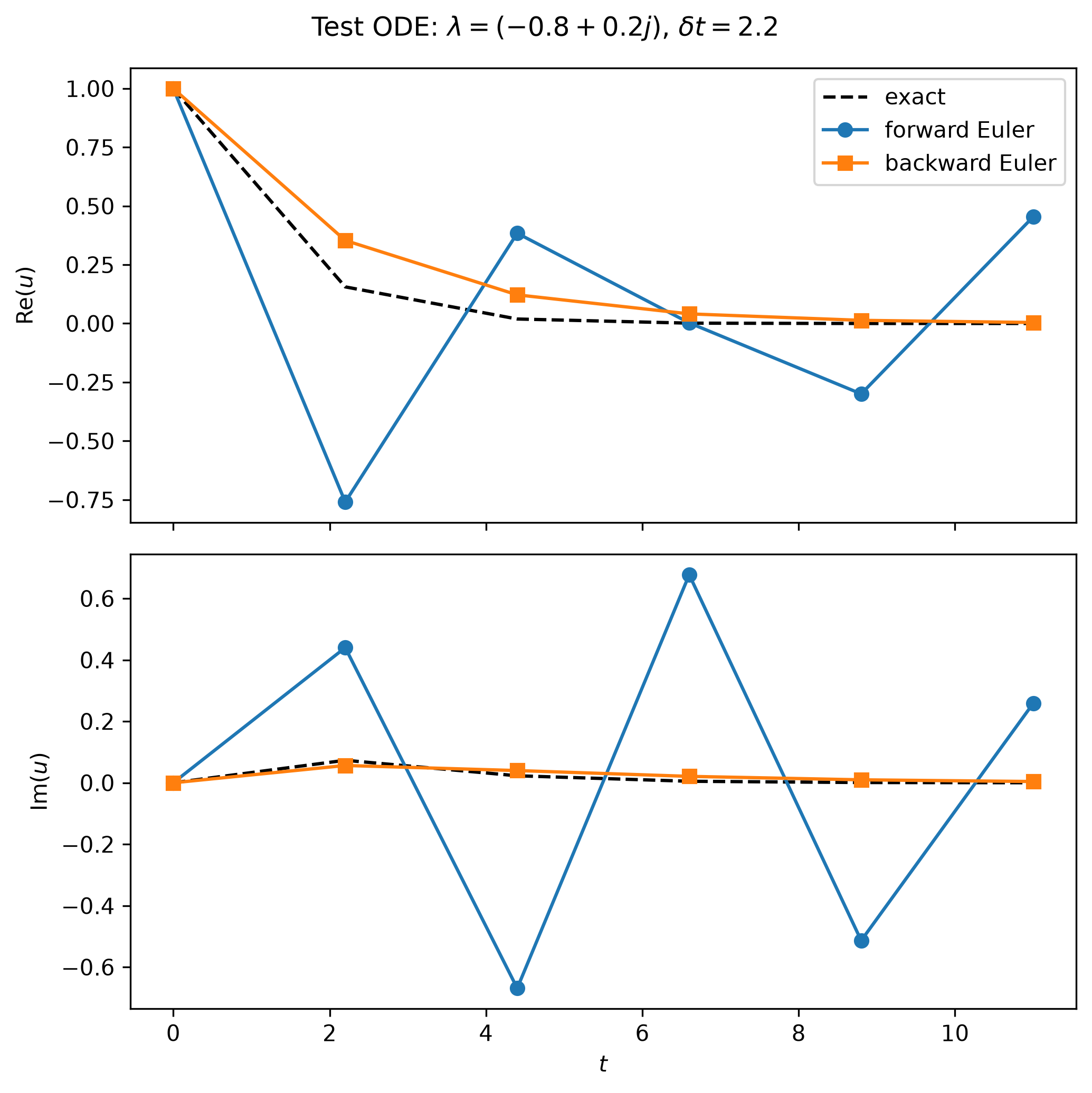
Forward and backward Euler on the test ODE. Left: \( \Delta t = 0.5 \). Right: \( \Delta t = 2.2 \).

With \( \Delta t = 0.5 \), both numerical solutions deviate a bit from the truth (expected, since we only solve approximately) but stay close and match its qualitative behavior. With \( \Delta t = 2.2 \) the picture changes: forward Euler exhibits large oscillations, while backward Euler remains more or less stable.

We’ll formalize stability later, but this is prototypical:

Explicit methods are often cheaper per iteration but can be unstable. Implicit methods are often more expensive but tend to be more stable.