Extension to Nonlinear Systems of ODEs#

Last time we introduced forward and backward Euler and tried them on the test ODE. Now for the practical details of using them on nonlinear problems and systems, plus some examples that motivate more advanced methods and a theoretical framework for analyzing them.

Solving Nonlinear ODEs with Backward Euler#

Consider a generic nonlinear (still scalar) ODE

Forward Euler doesn’t care: we only need to evaluate \( f \) at the known point \( (t_n, u_n) \) .

\begin{algorithm}
\caption{Forward Euler}
\begin{algorithmic}
\State Given $c$, $f$, $\Delta t$
\State Set $u_0 = c$
\For{$n = 0, 1, 2, \dots, T/\Delta t - 1$}
    \State Set $u_{n+1} = u_n + \Delta t \, f(t_n, u_n)$
\EndFor
\end{algorithmic}
\end{algorithm}

It’s a bit more complicated to write out backward Euler,

because \( f(t_{n+1}, u_{n+1}) \) is a general nonlinear function of the unknown, so we have to solve a nonlinear equation every step. Any nonlinear solver works, but our primary approach is Newton’s method.

Newton’s Method#

Consider

where \( g : \mathbb{R} \to \mathbb{R} \) is continuously differentiable. Our goal is to find \( v \). We build a sequence of guesses \( \{v_k\}_{k \geq 0} \) that should end up arbitrarily close to \( v \). At each guess, we pretend \( g \) is linear and solve for the root of its linear Taylor expansion

• We need to pick an initial guess \( v_0 \)
• We need to be able to evaluate \( g \) and \( g’ \)
• We assume \( g’ \) stays bounded away from zero near the solution

Convergence of Newton’s method is nontrivial and depends on the initialization and the smoothness of \( g \) (see e.g. Nocedal & Wright, Thm. 3.5).

So how does this help us with backward Euler? Let \( v = u_{n+1} \)

Notice that

so our Newton sub-iterations take the form

Typically we use \( v_0 = u_n \) as the initial guess, since \( u_{n+1} \to u_n \) as \( \Delta t \to 0 \). Newton converges (asymptotically) quadratically near the solution, so we only need a few iterations, but we never converge exactly. We stop when \( |v_{k+1} - v_k| < \text{tol} \) for some prescribed tolerance, e.g. \( 10^{-8} \).

\begin{algorithm}
\caption{Backward Euler with Newton Sub-iterations}
\begin{algorithmic}
\State Given $c$, $f$, $\Delta t$, and tolerance $\text{tol} > 0$
\State Set $u_0 = c$
\For{$n = 0, 1, 2, \dots, T/\Delta t - 1$}
    \State Initialize $v_0 = u_n$
    \State Set $k = 0$
    \Repeat
        \State Set $v_{k+1} = v_k - \dfrac{v_k - u_n - \Delta t \, f(t_{n+1}, v_k)}{1 - \Delta t \, \frac{\partial f}{\partial u}(t_{n+1}, v_k)}$
        \State Increment $k \gets k+1$
    \Until{$|v_{k+1} - v_k| < \text{tol}$}
    \State Set $u_{n+1} = v_{k+1}$
\EndFor
\end{algorithmic}
\end{algorithm}

Not too bad! Now we have nested loops, so the cost per step is waaaay higher, but it is at least stable.

Example: Growing Ice Thickness#

Stefan’s ice-growth law models the thickness \( u \) of ice on top of a frozen lake

where \( D > 0 \) is an effective thermal diffusivity of the ice. This has an analytic solution: the ODE is \( \dv{}{t} u^2 = 2D \), so

The ice grows like \( \sqrt{t} \): thickening slows down over time.

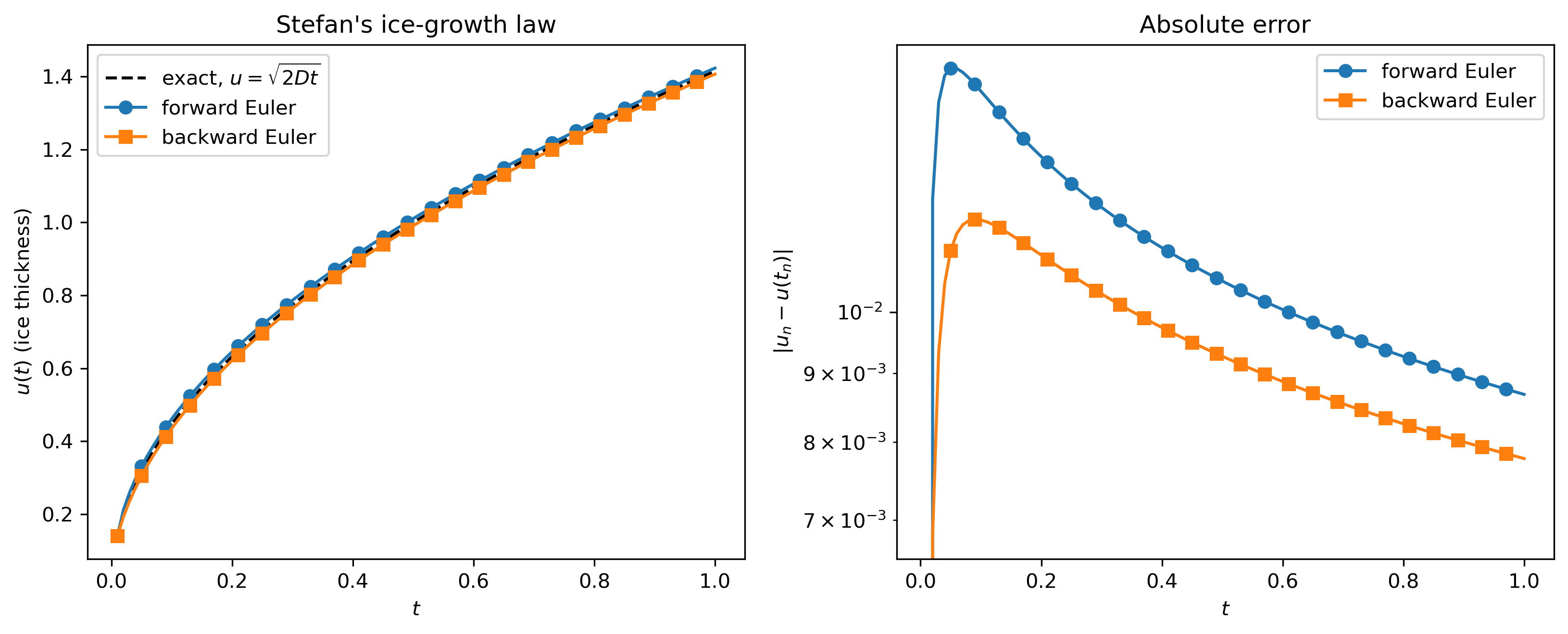
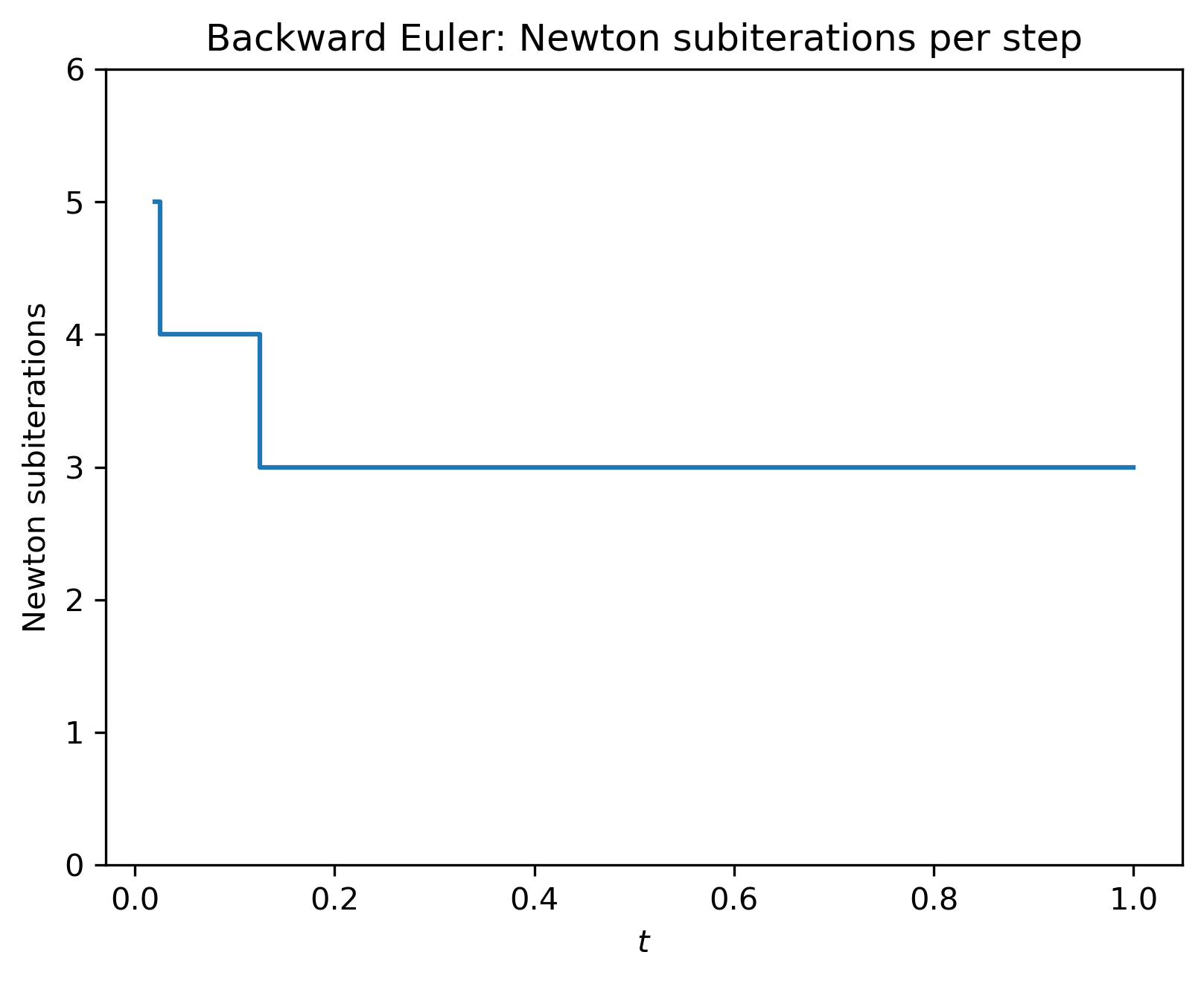
Stefan's ice-growth law, \( \Delta t = 0.01 \). Left: numerical solutions against the truth. Middle: errors. Right: Newton sub-iterations per step.

Systems of ODEs with Euler#

Forward Euler is exactly the same, just with vector-valued \( \vec{u} \)

But backward Euler

now requires solving a nonlinear system of equations at each step, so we extend Newton’s method to systems.

Newton’s Method for Systems#

Consider a generic problem

The Jacobian of \( \vec{g} \) is the matrix of partial derivatives, with the gradients of each component as its rows

Again this comes from a Taylor expansion of \( \vec{g} \)

Set the linear part to zero and solve for \( \vec{v}_{k+1} \)

Of course we don’t want to compute a whole inverse, so in practice we solve the linear system

For backward Euler, \( \vec{g}(\vec{v}) = \vec{v} - \vec{u}_n - \Delta t \, \vec{f}(t_{n+1}, \vec{v}) \) , so \( D\vec{g} = I - \Delta t \, D_{\vec{u}}\vec{f} \) and the sub-iterations are

We now need access to \( D\vec{f} \) and a linear solve every Newton iteration. \( D\vec{f} \) can be approximated many ways, though nowadays automatic differentiation is often used to compute it efficiently.

\begin{algorithm}
\caption{Backward Euler with Newton Sub-iterations for Systems}
\begin{algorithmic}
\State Given $\mathbf{c}$, $\mathbf{f}$, $D_{\mathbf{u}}\mathbf{f}$, $\Delta t$, and tolerance $\text{tol} > 0$
\State Set $\mathbf{u}_0 = \mathbf{c}$
\For{$n = 0, 1, 2, \dots, T/\Delta t - 1$}
    \State Initialize $\mathbf{v}_0 = \mathbf{u}_n$
    \State Set $k = 0$
    \Repeat
        \State Set $\mathbf{v}_{k+1} = \mathbf{v}_k - \left( I - \Delta t \, D_{\mathbf{u}} \mathbf{f}(t_{n+1}, \mathbf{v}_k) \right)^{-1} \left[ \mathbf{v}_k - \mathbf{u}_n - \Delta t \, \mathbf{f}(t_{n+1}, \mathbf{v}_k) \right]$
        \State Increment $k \gets k+1$
    \Until{$\| \mathbf{v}_{k+1} - \mathbf{v}_k \| < \text{tol}$}
    \State Set $\mathbf{u}_{n+1} = \mathbf{v}_{k+1}$
\EndFor
\end{algorithmic}
\end{algorithm}

Example: Predator-Prey Model (Lotka-Volterra)#

where \( u_1 \) is the prey population, \( u_2 \) is the predator population, and \( \alpha, \beta, \gamma, \delta > 0 \). The RHS and its Jacobian are

This gives us everything we need to plug and chug.

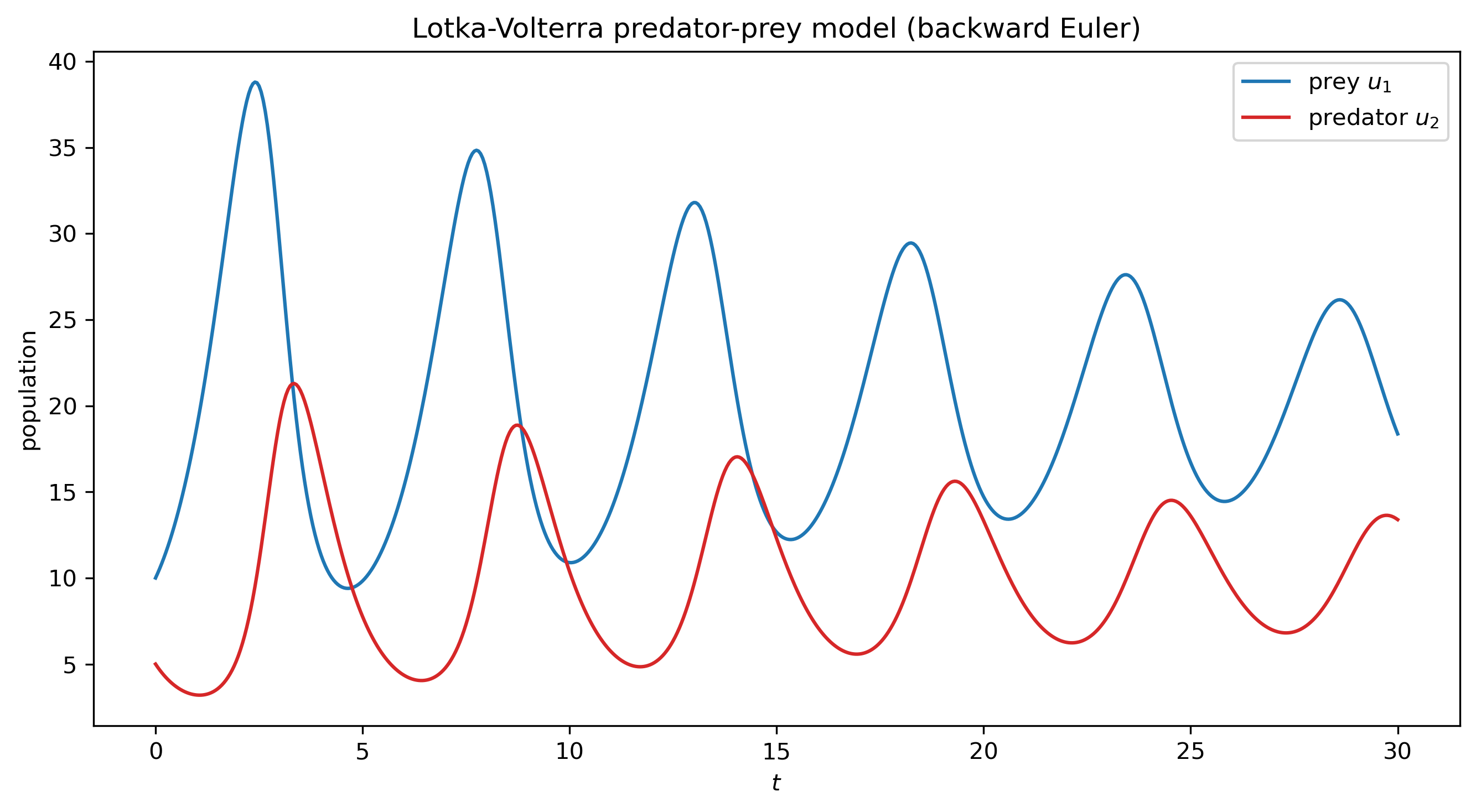
Lotka-Volterra with \( (\alpha, \beta, \gamma, \delta) = (1, 1, 1.5, 0.075) \), computed with backward Euler + Newton sub-iterations.