Accuracy#

We’ve noticed some peculiar things about Euler’s methods: on the test ODE the numerical solutions deviated from the truth, and in some regimes forward Euler went unstable while backward Euler didn’t. Let’s dig deeper, starting with convergence and numerical accuracy.

Convergence#

At the very least, our numerical scheme should converge to the true solution as the resolution increases, i.e. as the discretization size goes to zero.

Definition: Convergence of an ODE solver#

Consider an ODE with a ground truth solution \( u : [0, T] \to \mathbb{R} \), and an ODE solver that, for an integer \( N \), produces a sequence of approximations

\[u_n \approx u(t_n) \qquad t_n = n \Delta t \qquad n = 0, 1, \ldots, N \qquad \Delta t = \frac{T}{N}\]

We say that the method is convergent if

\[\lim_{\Delta t \to 0} \max_{0 \leq n \leq N} |u(t_n) - u_n| = 0\]

The definition can be adjusted for different purposes, e.g. if we only care about the final time we could ask for \( \lim_{\Delta t \to 0} |u(T) - u_N| = 0 \) . Note that convergence also depends on the ground truth: at the very least it has to be well-defined.

Empirically, convergence looks like the numerical solution approaching the truth as \( \Delta t \) shrinks. For forward Euler on the test ODE (real \( \lambda \)):

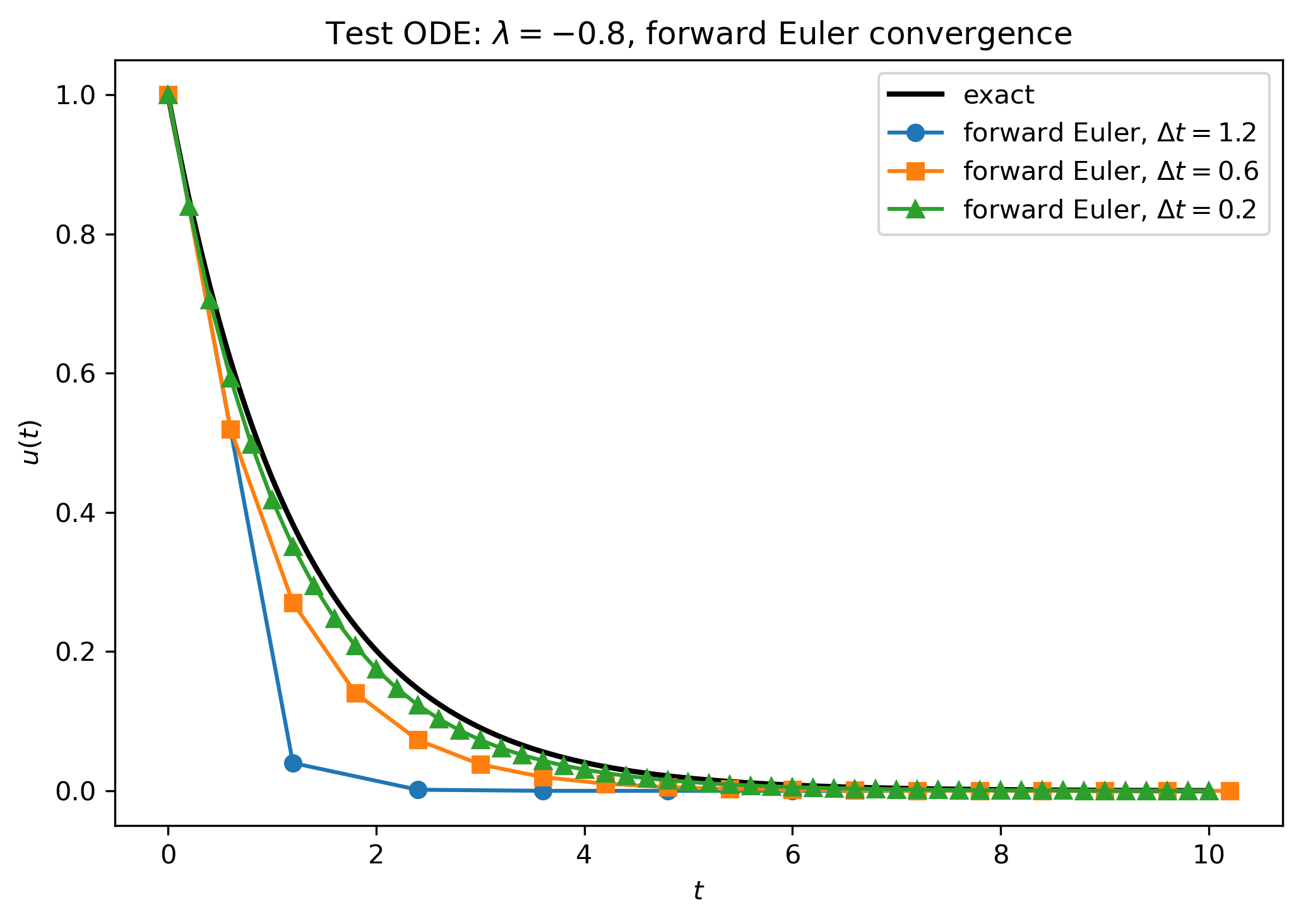
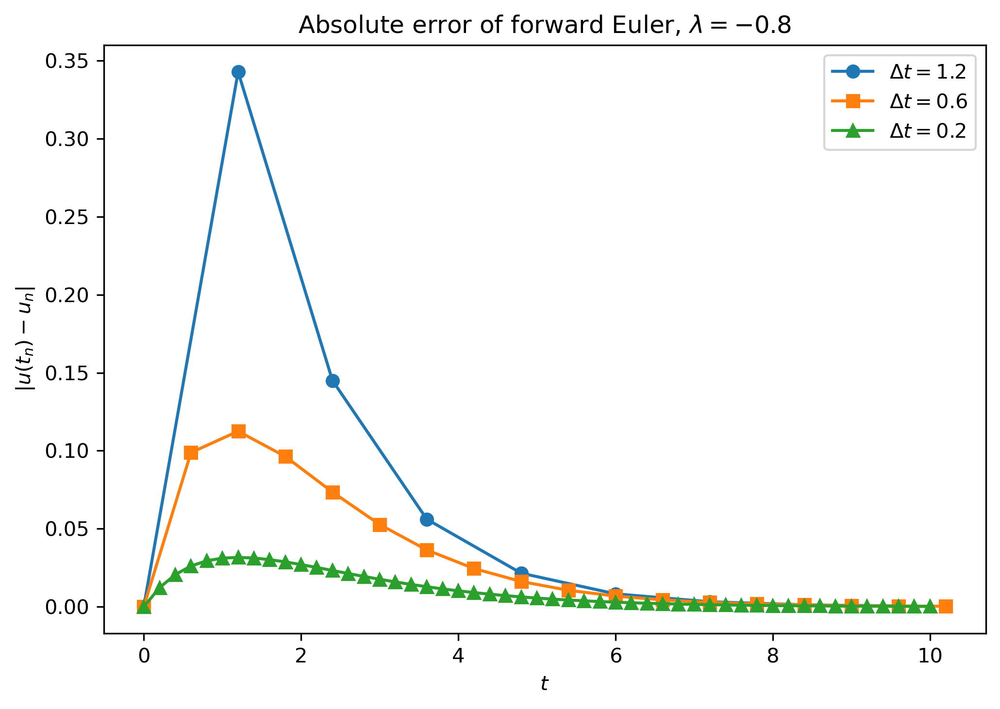
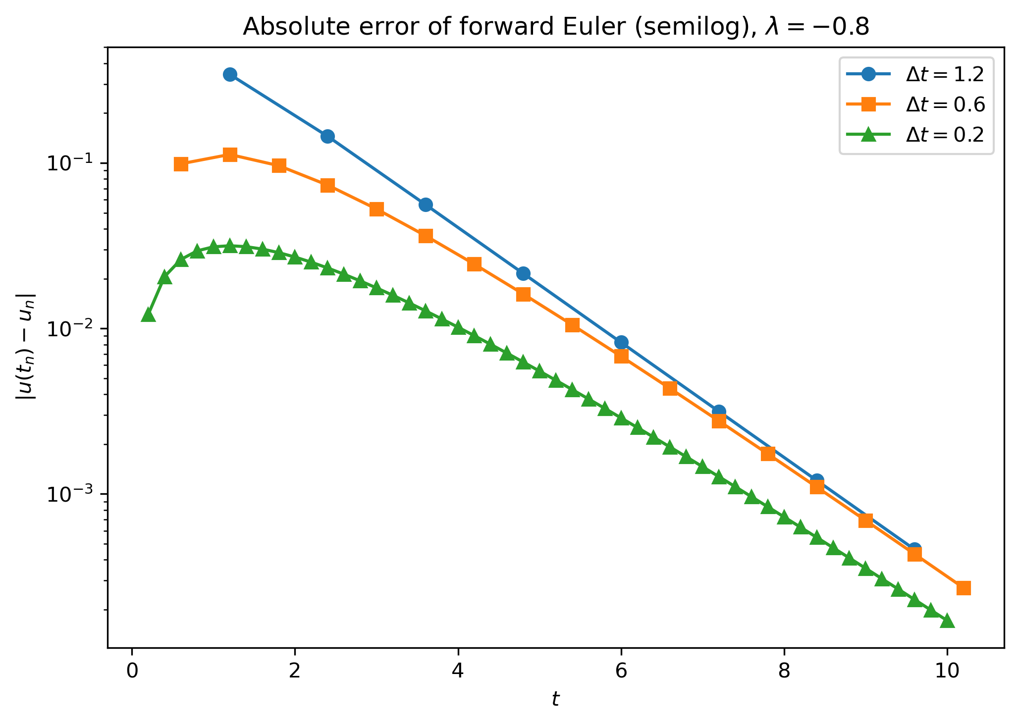
Left: numerical solutions approach the truth. Middle: errors \( |u(t_n) - u_n| \) shrink with \( \Delta t \). Right: the same errors on a semilog scale, which we routinely use since errors are small.

Numerical Accuracy#

Convergence alone is a pretty weak statement (though without it the algorithm is useless). It’s a more useful concept for comparing schemes if we consider the rate at which the limit goes to zero, i.e. how accurate the method is. We consider two types of error.

The global error is the difference between the true and numerical solutions

We usually look at \( |e_n| \), since the sign is less important than the magnitude.

The local truncation error asks: how close is the actual solution to satisfying the discretization of the ODE? I.e. it measures the error introduced by the scheme in a single step. For forward Euler this is

the residual of the discretized ODE after plugging in the true solution. We call \( \mathcal{N}_{\Delta t} \) the difference operator of the scheme. (The notation hides that \( \mathcal{N} \) depends on \( f \), \( t_{n-1} \) , and \( u(t_{n-1}) \) — think of it as an operator acting on \( u(t_n) \) with parameters that are known either as problem inputs or from previous steps.) Other schemes just use a different difference operator, e.g. for backward Euler

So global and local truncation errors fit in a unified framework for arbitrary ODE solvers. If you want something concrete to ground your reading, just keep forward Euler in mind. It’ll turn out the local truncation error is closely related to the global error.

Order of Accuracy and Convergence#

Following Ascher & Petzold:

Definition: Order of accuracy / convergence#

A scheme is accurate (or consistent) of order \( p \) if

\[\tau_n = \mathcal{O}(\Delta t^p) \qquad n = 1, 2, \ldots\]

A scheme is convergent of order \( p \) if

\[e_n = \mathcal{O}(\Delta t^p) \qquad n = 1, 2, \ldots\]

Disclaimer: order of convergence does not necessarily equal order of accuracy! BUT for every method we will be working with, they are equal. It’s usually easy to control the local truncation error and verify the order of accuracy.

Example: Euler Methods Are First-Order Accurate#

Both forward and backward Euler are first-order accurate (left as a homework assignment). Taylor expanding directly gives

Empirical Validation of the Order of Convergence#

It turns out both Euler methods are also first-order convergent. That’s harder to prove (see next lecture), but we can pretty convincingly show it empirically. If \( |e_n| \approx C \Delta t^p \), then

so the slope of \( \log |e_n| \) against \( \log \Delta t \) estimates \( p \). The recipe:

1. Pick a problem for which you have an analytic solution \( u(t) \)
2. Implement your method to obtain \( u_n \) for different choices of \( \Delta t \)
3. For each \( \Delta t \), compute the error \( |e_n| = |u(t_n) - u_n| \)
4. Plot \( \log |e_n| \) against \( \log \Delta t \) and check that the slope is \( p \)

Since the error bound holds uniformly in \( n \), it’s usually sufficient to use \( \max_n |e_n| \) . The average \( \frac{1}{N} \sum_n |e_n| \) also works and gives the same rate for ODE solvers — but for other kinds of algorithms the average rate can be better than the max rate, so be careful interpreting it.

For example, forward Euler on Stefan’s ice-growth problem, with exact solution \( u(t) = \sqrt{2Dt + c^2} \):

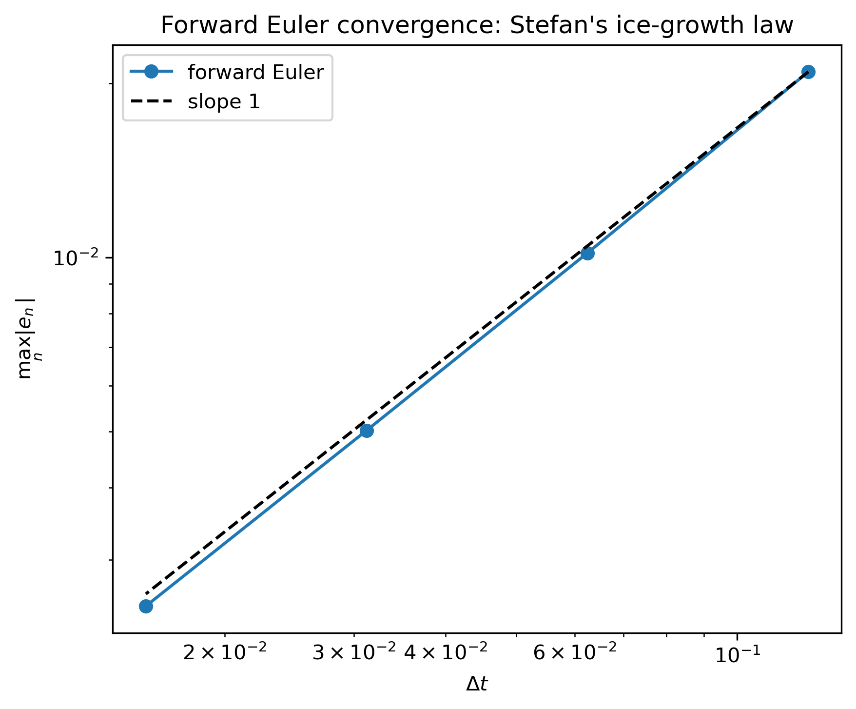
\( \max_n |e_n| \) against \( \Delta t \) for forward Euler on Stefan's ice-growth problem.

Trapezoid Method#

Let’s take a look at our first second-order accurate scheme, the (symmetric) trapezoid method

This is implicit, since \( f(t_n, u_n) \) appears on the right-hand side. For the truncation error, it helps to Taylor expand about the midpoint \( t_{n-1/2} = \frac{1}{2}(t_{n-1} + t_n) \)

Subtracting, the even terms cancel

To make this useful, we need \( u'(t_{n-1/2}) \) in terms of the endpoints, so expand \( u’ \) about \( t_{n-1/2} \) in both the \( +\frac{\Delta t}{2} \) and \( -\frac{\Delta t}{2} \) directions

Averaging, now the odd terms cancel

and since \( u’ = f(t, u) \) for the true solution, all together

So the trapezoid method is \( 2^{\text{nd}} \)-order accurate.

Keep in mind, we needed to assume \( u \) is sufficiently smooth (three times continuously differentiable) to show this. The method won’t achieve this order of accuracy if e.g. \( u’’’ \) is not bounded.