Absolute Stability#
In Accuracy we introduced convergence and numerical accuracy. A convergent algorithm is the minimum we need for it to be useful: eventually, with enough computing power (small \( \Delta t \)), it gives a good approximation to the truth. An order of convergence makes this much stronger, since it tells us exactly how fast the error decays. But accuracy alone isn’t quite sufficient to make a method useful, and there’s a tension between accuracy and stability.
Absolute Stability on the Test ODE#
Recall the test ODE
\[\dv{u}{t} = \lambda u \qquad u(0) = c\]and the experiment where forward Euler oscillated wildly for large \( \Delta t \) while backward Euler stayed stable. This behavior is so fundamental that the mathematical definition of stability is usually built around the test ODE itself.
The exact solution is \( u(t) = c e^{\lambda t} \), so if \( \text{Re}(\lambda) < 0 \) the solution decays to zero as \( t \to \infty \). Applying forward Euler,
\[u_n = u_{n-1} + \Delta t \lambda u_{n-1} = (1 + \Delta t \lambda) u_{n-1}\]and substituting recursively,
\[u_n = (1 + \Delta t \lambda)^n u_0\]So the numerical solution decays to zero if and only if
\[|1 + \Delta t \lambda| < 1\]If \( \lambda \) is real and negative, this is
\[-1 < 1 + \Delta t \lambda < 1 \quad \Rightarrow \quad \Delta t < \frac{2}{-\lambda} = \frac{2}{|\lambda|} \equiv \Delta t_{\max}\]So there’s a limit on the size of \( \Delta t \) if we want the numerical solution to decay like the true one. For complex \( \lambda \), the condition says \( \Delta t \lambda \) has to lie inside the disk of radius 1 centered at \( -1 \).
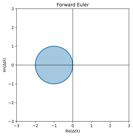
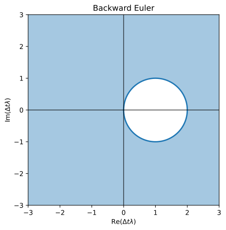
Regions of absolute stability (shaded) in the \( z = \lambda \Delta t \) plane. Left: forward Euler. Right: backward Euler.
Why the Test ODE?#
Why do we care about this particular problem decaying to zero? Suppose we’ve computed \( \{u_n\}_{n=0}^{N-k} \) with forward Euler, and a small perturbation gets into the last estimate, \( u_{N-k} \leftarrow u_{N-k} + \epsilon \) . This happens all the time due to round-off error. Forward Euler then continues with
\[u_{\epsilon, N-k+j} = (1 + \Delta t \lambda)^j (u_{N-k} + \epsilon) \qquad j = 1, 2, \ldots, k\]so the error \( \delta u_{N-k+j} = u_{\epsilon, N-k+j} - u_{N-k+j} \) satisfies
\[\delta u_{N-k+j} = (1 + \Delta t \lambda)^j \epsilon \qquad j = 1, 2, \ldots, k\]We’d prefer this perturbation not grow. The amplification factor \( (1 + \Delta t \lambda) \) is the same one that governs the solution itself.
Why Only the Linear ODE?#
How does this relate to stability for nonlinear problems? Consider
\[\dv{u}{t} = f(u) \qquad u(0) = c\]with true solution \( u(t) \). Suppose we make small errors, in the initial condition or in evaluating \( f \), giving a perturbed solution \( v(t) = u(t) + \epsilon(t) \). Substituting into the ODE,
\[\dv{\epsilon}{t} = f(u + \epsilon) - f(u) = \pdv{f}{u}(u) \, \epsilon + \text{higher order terms}\]So, roughly, the perturbation solves a linear ODE like the test ODE, except the coefficient \( \lambda \to \partial f / \partial u (u(t)) \) depends on time. At least over short time intervals, the perturbation stays controlled if
\[\left| 1 + \Delta t \pdv{f}{u}(u) \right| \leq 1\]Formal Definitions#
Definition: Absolute stability#
Consider the test ODE with \( \lambda \in \mathbb{C} \), \( \text{Re}(\lambda) < 0 \). Suppose \( \{u_n\}_{n=0}^{\infty} \) is a numerical solution produced by an ODE solver. The solution is absolutely stable if
\[|u_n| \leq |u_{n-1}| \qquad n = 1, 2, \ldots\]
Definition: Region of absolute stability#
For a given method, the region of absolute stability is the set of all \( z = \lambda \Delta t \in \mathbb{C} \) for which the numerical solution of the test ODE is absolutely stable.
For forward Euler this region is \( \{ z \in \mathbb{C} : |1 + z| \leq 1 \} \) , and for backward Euler (below) it’s \( \{ z \in \mathbb{C} : |1 - z| \geq 1 \} \) .
Definition: A-stability#
A method is A-stable if its region of absolute stability contains the entire left half of the complex plane, \( \text{Re}(z) < 0 \).
So forward Euler is not A-stable, while backward Euler is.
Stability of Backward Euler#
We can finally make sense of the difference we saw between forward and backward Euler. Applying backward Euler to the test ODE,
\[u_n = u_{n-1} + \Delta t \lambda u_n \quad \to \quad u_n = (1 - \Delta t \lambda)^{-1} u_{n-1}\]so
\[|u_n| = \left| (1 - \Delta t \lambda)^{-1} \right| |u_{n-1}|\]If \( \text{Re}(\lambda) < 0 \), then \( |1 - \Delta t \lambda| \geq \text{Re}(1 - \Delta t \lambda) = 1 - \Delta t \, \text{Re}(\lambda) > 1 \) , so the amplification factor is less than 1. Backward Euler is absolutely stable for any \( \Delta t > 0 \) whenever \( \text{Re}(\lambda) < 0 \). Its region of absolute stability is the whole complex plane minus the open disk of radius 1 centered at \( +1 \).
This has profound practical implications: we can take as large a step as we want without worrying about instabilities.
Stability does not mean accuracy! Large time steps still give larger errors. Stability only ensures that perturbations don’t grow uncontrollably.