Stability for Systems and Stiffness#
Two more topics: extending absolute stability to systems of ODEs, and stiffness, which sits at the intersection of stability and accuracy.
Stability for Systems#
We extend absolute stability to systems by considering the test problem
\[\dv{\vec{u}}{t} = A \vec{u} \qquad \vec{u}(0) = \vec{c}\]where we assume \( A \) is diagonalizable, so
\[A = Q \Lambda Q^{-1}\]with \( Q \in \mathbb{C}^{d \times d} \) the matrix of eigenvectors and \( \Lambda \in \mathbb{C}^{d \times d} \) the diagonal matrix of eigenvalues. Multiplying the ODE by \( Q^{-1} \) and letting \( \vec{z}(t) = Q^{-1} \vec{u}(t) \),
\[\dv{\vec{z}}{t} = \Lambda \vec{z} \qquad \vec{z}(0) = Q^{-1} \vec{c}\]Since \( \Lambda \) is diagonal, the system decouples into \( d \) independent scalar test ODEs
\[\dv{z_i}{t} = \lambda_i z_i \qquad z_i(0) = (Q^{-1} \vec{c})_i\]so everything we know about absolute stability for scalar ODEs applies to each mode. (This works for forward and backward Euler because both commute with the change of variables: e.g. \( \vec{u}_n = (I + \Delta t A)\vec{u}_{n-1} \) becomes \( \vec{z}_n = (I + \Delta t \Lambda)\vec{z}_{n-1} \) .)
For forward Euler, we need \( |1 + \Delta t \lambda_i| \leq 1 \) for every \( i = 1, \ldots, d \). When the \( \lambda_i \) are real and negative,
\[0 < \Delta t \leq \frac{2}{\max_i |\lambda_i|}\]so the stability restriction is dictated by the eigenvalue of \( A \) with the largest magnitude.
For backward Euler we need \( |1 - \Delta t \lambda_i|^{-1} \leq 1 \) , i.e. \( |1 - \Delta t \lambda_i| \geq 1 \) , for every \( i \), which holds for any \( \Delta t > 0 \) whenever all \( \text{Re}(\lambda_i) < 0 \) . So backward Euler is still A-stable for systems.
Stiffness#
Stiffness reveals a tension between stability and accuracy. It’s somewhat qualitative, so it’s best described by example.
Example: A Stiff Scalar ODE#
\[\dv{u}{t} = -100 \left( u - \sin(t) \right) \qquad u(0) = 1 \qquad t \geq 0\]Because of the \( -100 \), the solution initially decays very rapidly toward \( \sin(t) \), which is near zero for small \( t \). After this transient, the sinusoid dominates the behavior of the solution.
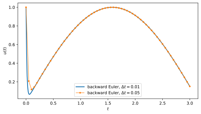
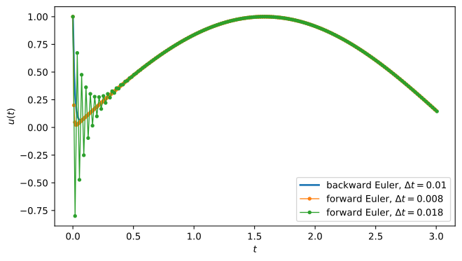
The stiff ODE solved with backward Euler (left) and forward Euler (right), against \( \sin(t) \), the dominant mode after the initial transient.
Backward Euler stays stable, as expected, even for large \( \Delta t \). Forward Euler goes unstable roughly when \( \Delta t > 2/100 = 0.02 \), the limit set by \( \lambda = -100 \) (the Jacobian \( \partial f / \partial u \)).
This is the typical picture of a stiff problem: a severe restriction is imposed on explicit methods like forward Euler, but the fast dynamics responsible only matter for a brief period. Once the transient has passed, the solution could be approximated well with much larger time steps, but the explicit method is still stuck with the small \( \Delta t \) for stability. Implicit methods like backward Euler are unconditionally stable, so they handle the stiff phase without excessively small time steps.
Example: A Stiff Linear System#
Stiffness also shows up in systems, where some coordinates have large eigenvalues (fast dynamics) and others have small eigenvalues (slow dynamics). The fast coordinates impose a severe time-step restriction on explicit methods, even though the slow coordinates could be advanced with much larger steps.
\[\dv{u_1}{t} = -u_1 \qquad \dv{u_2}{t} = -\lambda (u_2 - u_1) \qquad \left(u_1(0), u_2(0)\right) = (c_1, c_2)\]In matrix form,
\[\dv{}{t} \begin{bmatrix} u_1 \\ u_2 \end{bmatrix} = \underbrace{\begin{bmatrix} -1 & 0 \\ \lambda & -\lambda \end{bmatrix}}_{A} \begin{bmatrix} u_1 \\ u_2 \end{bmatrix}\]\( A \) is lower triangular, so its eigenvalues are \( -1 \) and \( -\lambda \). If \( \lambda \gg 1 \), the second equation has a much faster timescale than the first and the system is stiff. Solving analytically,
\[u_1(t) = c_1 e^{-t} \qquad u_2(t) = \frac{\lambda c_1}{\lambda - 1} e^{-t} + \left( c_2 - \frac{\lambda c_1}{\lambda - 1} \right) e^{-\lambda t}\]For \( \lambda \gg 1 \), \( u_2 \) is pulled toward \( u_1 \) very quickly (the \( e^{-\lambda t} \) transient), while \( u_1 \) itself evolves slowly. Forward Euler still needs \( \Delta t \leq 2/\lambda \) for the entire simulation, even after the fast mode has died out.
Stiffness Ratio#
For a linear system, stiffness can be characterized by the stiffness ratio: the ratio of the largest to the smallest eigenvalue magnitude of the system matrix,
\[\frac{\max_i |\lambda_i|}{\min_i |\lambda_i|}\]A large stiffness ratio means the system has widely varying timescales. For nonlinear ODEs, we look at the eigenvalues of the Jacobian \( D_{\vec{u}}\vec{f} \) in the same way, keeping in mind that the Jacobian changes as the solution evolves.
The practical message: if a problem is stiff, it’s worth paying the extra computational cost of an implicit method like backward Euler, or another solver specialized for stiffness.