Higher Order Methods I: The Runge-Kutta Family#

So far we’ve mostly used forward and backward Euler, both first-order consistent and convergent. We usually just say they’re first-order accurate, meaning both the local truncation and global errors are \( \mathcal{O}(\Delta t) \). They’re simple, but in practice we’d like methods with accuracy \( \mathcal{O}(\Delta t^p) \) for, say, \( p = 2 \) or \( p = 4 \). With a second-order method, halving the step size \( \Delta t \leftarrow \Delta t / 2 \) cuts the error by a factor of \( 2^2 = 4 \). With a fourth-order method it drops by a factor of 16! These methods can really pay off.

This lecture covers one-step methods, where \( \vec{u}_n \) is computed only from \( \vec{u}_{n-1} \) . Next up are multistep methods, where \( \vec{u}_n \) is computed from several previous values \( \vec{u}_{n-1}, \vec{u}_{n-2}, \ldots, \vec{u}_{n-k} \) .

Quadrature#

Our starting point for deriving higher-order methods is the approximation of integrals, called quadrature. For some function \( g : [a, b] \to \mathbb{R} \), pick \( s \) distinct points \( x_1, \ldots, x_s \in [a, b] \) and weights \( w_1, \ldots, w_s \) and approximate

The choice of points and weights \( (x_i, w_i) \) is the quadrature rule. Popular examples:

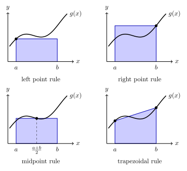
The four quadrature rules applied to a smooth \( g \). The shaded area is what the rule computes; the exact integral is the area under \( g(x) \). Dots mark where \( g \) is evaluated.

From Quadrature to ODE Solvers#

Take a generic scalar ODE, switching to prime notation \( u’(t) = \dv{u}{t}(t) \) for convenience,

(the methods extend naturally to systems). Integrate both sides over \( [t_{n-1}, t_n] \) :

Each quadrature rule for the right-hand side gives a time-stepping scheme.

• Left point rule \( \to \) forward Euler:

• Right point rule \( \to \) backward Euler:

• Trapezoidal rule \( \to \) the trapezoid method from before:

• Midpoint rule:

This needs \( u(t_{n-1/2}) \), which we don’t have. There are two ways to approximate it.

Implicit Midpoint#

Approximate \( u(t_{n-1/2}) \) by the average of \( u(t_{n-1}) \) and \( u(t_n) \) :

Explicit Midpoint (RK2)#

Alternatively, approximate \( u(t_{n-1/2}) \) with an intermediate forward Euler half-step:

This is our first Runge-Kutta method, sometimes called RK2.

The Runge-Kutta idea: construct a series of intermediate approximations to the solution within each step in order to improve the order of accuracy.

\begin{algorithm}
\caption{Explicit Midpoint (RK2)}
\begin{algorithmic}
\State Given $c$, $f$, $\Delta t$
\State Set $u_0 = c$
\For{$n = 1, 2, \dots, T/\Delta t$}
    \State Set $\hat{u}_{n-1/2} = u_{n-1} + \frac{\Delta t}{2} f(t_{n-1}, u_{n-1})$
    \State Set $u_n = u_{n-1} + \Delta t \, f(t_{n-1/2}, \hat{u}_{n-1/2})$
\EndFor
\end{algorithmic}
\end{algorithm}

RK2 Is Second-Order Accurate#

The point of the extra stage is that the resulting explicit scheme is second-order accurate. Plug the true solution into the scheme:

Expand everything about \( t_{n-1} \) . Below, \( u, u’, \ldots \) and \( f, f_t, f_u, \ldots \) are all evaluated at \( t_{n-1} \) , \( (t_{n-1}, u(t_{n-1})) \) . The first term is

The second term is \( f \) evaluated at a point shifted by \( \left(\frac{\Delta t}{2}, \frac{\Delta t}{2} f\right) \), so a 2D Taylor expansion gives

Differentiating the ODE \( u’ = f(t, u) \) along the solution with the chain rule,

Substituting, the \( \mathcal{O}(1) \) and \( \mathcal{O}(\Delta t) \) terms cancel exactly, leaving

It can also be shown that the method is 0-stable, so by the Lax equivalence theorem it’s second-order convergent.

Classical Fourth-Order Runge-Kutta (RK4)#

Continuing this line of thinking with more accurate quadrature rules gives higher-order Runge-Kutta methods. The most popular is the classical fourth-order Runge-Kutta method (RK4), widely used in off-the-shelf solvers:

The final update is Simpson’s rule, \( \int_a^b g \approx \frac{b-a}{6}\left(g(a) + 4 g\left(\tfrac{a+b}{2}\right) + g(b)\right) \) , with the midpoint value split between two estimates. The intermediate values \( \hat{u}_i \) are just forward Euler approximations built from the previous estimates. Even though forward Euler is only first-order accurate, the combination ends up fourth-order accurate.

\begin{algorithm}
\caption{Classical Runge-Kutta (RK4)}
\begin{algorithmic}
\State Given $c$, $f$, $\Delta t$
\State Set $u_0 = c$
\For{$n = 1, 2, \dots, T/\Delta t$}
    \State $k_1 = f(t_{n-1}, u_{n-1})$
    \State $k_2 = f(t_{n-1/2}, u_{n-1} + \frac{\Delta t}{2} k_1)$
    \State $k_3 = f(t_{n-1/2}, u_{n-1} + \frac{\Delta t}{2} k_2)$
    \State $k_4 = f(t_n, u_{n-1} + \Delta t \, k_3)$
    \State Set $u_n = u_{n-1} + \frac{\Delta t}{6} (k_1 + 2 k_2 + 2 k_3 + k_4)$
\EndFor
\end{algorithmic}
\end{algorithm}

(Here \( k_i = f(\cdot, \hat{u}_i) \) are the stage slopes. This is the more common way to write RK4.)

Stability of Explicit Runge-Kutta Methods#

Since these methods are all explicit, we expect stability restrictions. Applying them to the test ODE \( u’ = \lambda u \) with \( z = \lambda \Delta t \), each step multiplies by a polynomial amplification factor \( u_n = R(z) \, u_{n-1} \) . For RK2,

and similarly RK4 gives \( R(z) = 1 + z + \frac{z^2}{2} + \frac{z^3}{6} + \frac{z^4}{24} \): the Taylor series of \( e^z \), truncated at the order of the method. The region of absolute stability is \( \{ z : |R(z)| \leq 1 \} \) .

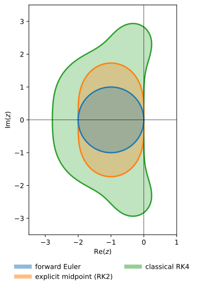
Stability regions for forward Euler, explicit midpoint (RK2), and RK4.

The regions grow with the order, but since \( R(z) \) is a polynomial, \( |R(z)| \to \infty \) as \( |z| \to \infty \): no explicit Runge-Kutta method is A-stable.