Finite Difference Methods#
Motivated by the Poisson example, we now outline the general framework of finite difference methods (FDMs) for solving BVPs.
General Structure of a Finite Difference Method#
FDMs for BVPs share a common three-step structure:
- Pick a grid (mesh): a set of points \( \{t_0, \ldots, t_N\} \subset [a, b] \)
- Discretize the differential equation using difference formulae
- Assemble and solve a linear or nonlinear system of algebraic equations
Example: Poisson’s Equation#
We already did these steps for the toy BVP
\[u''(t) = f(t) \qquad u(0) = c_0 \qquad u(1) = c_1\]Recalling them for context:
- Grid: a uniform grid on \( [0, 1] \), \( t_n = n \Delta t \) for \( n = 0, 1, \ldots, N \), \( \Delta t = 1/N \).
- Discretize: The Dirichlet boundary conditions need no approximation, so we only discretize \( u’’ \). With \( u_n \approx u(t_n) \) ,
- Assemble and solve: Substituting into the BVP and combining with the boundary conditions,
Write this as a matrix equation \( A \vec{u} = \vec{f} \) and compute \( \vec{u} = A^{-1} \vec{f} \).
Below we use homogeneous Dirichlet conditions and a smooth Gaussian bump \( f(t) = -\exp\left(-\frac{(t - 1/2)^2}{2\sigma^2}\right) \) with \( \sigma = 0.1 \), for which there’s an analytic solution. That lets us plot the error \( e_N = \max_n |u_n - u(t_n)| \) against the number of grid points \( N \).
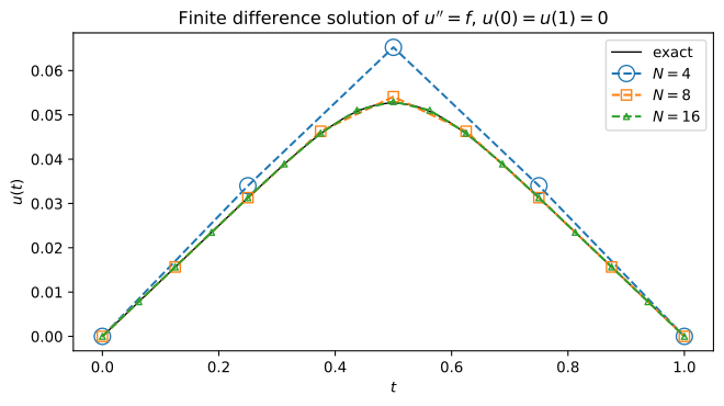
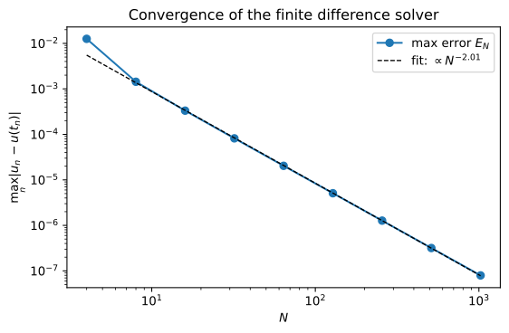
Left: FDM solutions of \( u'' = f \) for several \( N \). Right: the maximum error decays quadratically in the number of grid points.
We see \( e_N = \mathcal{O}(N^{-2}) = \mathcal{O}(\Delta t^2) \) . That’s not surprising, since the centered difference for \( u’’ \) is second-order accurate:
\[\frac{1}{\Delta t^2} \left( u(t_{n-1}) - 2u(t_n) + u(t_{n+1}) \right) = u''(t_n) + \frac{\Delta t^2}{12} u''''(t_n) + \mathcal{O}(\Delta t^4)\]Example: Advection-Diffusion#
The choice of difference formulae is what distinguishes different FDMs. Consider a more general second-order BVP, with an added first-derivative term:
\[-u''(t) + 2u'(t) = f(t) \qquad u(0) = u(1) = 0\]with \( f(t) = \exp\left(-\frac{(t - 1/2)^2}{2\sigma^2}\right) \) , \( \sigma = 0.1 \).
- Grid: as before, \( t_n = n \Delta t \), \( \Delta t = 1/N \).
- Discretize: the same centered difference for \( u’’ \), but a forward difference (as in forward Euler) for \( u’ \):
- Assemble and solve: Let \( A \) be the centered difference matrix from before, and define the forward difference matrix for the \( u’ \) term,
Then solve \( D \vec{u} = \vec{f} \) with \( D = -A + 2B \).
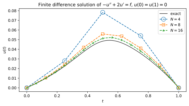
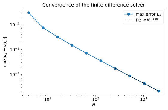
The same experiment for \( -u'' + 2u' = f \). The rate of convergence is now 1 rather than 2.
This time convergence is slower: only \( \mathcal{O}(N^{-1}) = \mathcal{O}(\Delta t) \) , so the method is first-order convergent. As we’ll see, this is because the first-order approximation of \( u’ \) limits the convergence rate of the whole algorithm, even though \( u’’ \) is approximated to second order.
Error Analysis for BVP Solvers#
Let’s justify the \( \mathcal{O}(\Delta t^2) \) convergence for the Poisson example. Define the truncation error, the residual of the discretized ODE after plugging in the true solution,
\[\tau_n = \frac{u(t_{n-1}) - 2u(t_n) + u(t_{n+1})}{\Delta t^2} - f(t_n)\]and the global error
\[e_n = u(t_n) - u_n\]just as for IVP solvers. Since \( u_n \) solves the discrete problem,
\[\frac{u_{n-1} - 2u_n + u_{n+1}}{\Delta t^2} - f(t_n) = 0\]Subtracting this from the definition of \( \tau_n \),
\[\tau_n = \frac{e_{n-1} - 2e_n + e_{n+1}}{\Delta t^2} \qquad n = 1, \ldots, N-1\]At the boundaries \( u_0 = u(t_0) = c_0 \) and \( u_N = u(1) = c_1 \) exactly, so
\[e_0 = e_N = 0\]Writing \( \vec{e} = (e_1, \ldots, e_{N-1}) \) and \( \vec{\tau} = (\tau_1, \ldots, \tau_{N-1}) \) ,
\[A \vec{e} = \Delta t^2 \vec{\tau} \quad \Rightarrow \quad \vec{e} = \Delta t^2 A^{-1} \vec{\tau} \qquad A = \begin{bmatrix} -2 & 1 & 0 & & \cdots & 0 \\ 1 & -2 & 1 & 0 & \cdots & 0 \\ 0 & 1 & -2 & 1 & \cdots & 0 \\ & & \ddots & \ddots & \ddots & \\ 0 & \cdots & 0 & 1 & -2 & 1 \\ 0 & \cdots & & 0 & 1 & -2 \end{bmatrix} \in \mathbb{R}^{(N-1) \times (N-1)}\]Note this \( A \) is the interior block without the \( 1/\Delta t^2 \) scaling. Taking norms,
\[\| \vec{e} \|_\infty \leq \Delta t^2 \, \| A^{-1} \|_\infty \, \| \vec{\tau} \|_\infty\]where for a vector \( \| \vec{x} \|_\infty = \max_j |x_j| \) , and the induced matrix norm is the maximum absolute row sum
\[\| A \|_\infty = \max_{\vec{x} \neq 0} \frac{\| A \vec{x} \|_\infty}{\| \vec{x} \|_\infty} = \max_i \sum_j |a_{ij}|\]It can be shown that \( \| A^{-1} \|_\infty \leq N^2/4 \) . (In fact \( \| A^{-1} \|_\infty = N^2/8 \) exactly for even \( N \): row \( i \) of \( |A^{-1}| \) sums to \( i(N - i)/2 \), the discrete analogue of the Green’s function for \( u’’ \).) Since \( \Delta t = 1/N \),
\[\| \vec{e} \|_\infty \leq \frac{1}{N^2} \cdot \frac{N^2}{4} \| \vec{\tau} \|_\infty = \frac{1}{4} \| \vec{\tau} \|_\infty\]We already know \( |\tau_n| = \mathcal{O}(\Delta t^2) \) , so \( \| \vec{\tau} \|_\infty = \mathcal{O}(\Delta t^2) \) and therefore
\[\| \vec{e} \|_\infty = \mathcal{O}(\Delta t^2)\]This is the BVP version of “consistency + stability = convergence”. The truncation error gives consistency, and a bound on \( \| A^{-1} \|_\infty \) that doesn’t blow up faster than \( 1/\Delta t^2 \) plays the role of stability: it stops the local errors from being amplified.