Solving a Variable Coefficient Second Order BVP#
Here we derive a second-order FDM for a variable coefficient BVP. Beyond the toy examples so far, this shows most of the considerations and ideas involved in solving a linear second-order BVP. Consider
\[-\dv{}{t} \left( a(t) \dv{u}{t}(t) \right) + b(t) \dv{u}{t}(t) + c(t) u(t) = f(t) \qquad t \in (0, 1)\]where \( a, b, c, f \) are given functions, subject to the Robin boundary conditions
\[a(0) \dv{u}{t}(0) = \alpha_0 u(0) + \beta_0 \qquad a(1) \dv{u}{t}(1) = \alpha_1 u(1) + \beta_1\]with given coefficients \( \alpha_0, \alpha_1, \beta_0, \beta_1 \) . We follow the usual three steps.
Step 1: A Uniform Grid#
Use a uniform grid on \( [0, 1] \), \( t_j = j \Delta t \) for \( j = 0, \ldots, N \), \( \Delta t = 1/N \). Later we’ll augment it with a pair of so-called ghost points, \( t_{-1} = -\Delta t \) and \( t_{N+1} = 1 + \Delta t \) , which help impose derivative conditions at the boundary.

The uniform grid on \( [0, 1] \). Boundary points \( t_0 = 0 \) and \( t_N = 1 \) are large dots; the ghost points \( t_{-1} \) and \( t_{N+1} \) are crosses.
Step 2: Discretize the BVP#
We replace every differential operator with a second-order accurate difference formula.
The Zeroth-Order Term#
This one is trivial:
\[c(t_j) u(t_j) \approx c_j u_j \qquad c_j = c(t_j)\]The First-Order Term#
For \( b u’ \) we only need to approximate \( u’ \), and we use the second-order centered difference
\[b(t_j) \dv{u}{t}(t_j) = b(t_j) \frac{u(t_{j+1}) - u(t_{j-1})}{2\Delta t} + \mathcal{O}(\Delta t^2) \approx b_j \frac{u_{j+1} - u_{j-1}}{2\Delta t} \qquad b_j = b(t_j)\]The Second-Order Term#
For \( (a u’)’ \) we need some care, since we’d prefer not to differentiate the coefficient \( a \). Instead, apply the centered difference twice, with the coefficient sampled on the staggered grid of midpoints \( t_{j \pm 1/2} = t_j \pm \Delta t/2 \) .
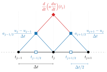
The stencil around \( t_j \). Level 1 (middle row): grid values \( u_{j-1}, u_j, u_{j+1} \) are combined to approximate \( a u' \) at the midpoints \( t_{j \pm 1/2} \), where \( a \) is sampled (hollow squares). Level 2 (top): the midpoint values are combined to approximate \( (a u')' \) at \( t_j \).
Level 1. Centered differences estimate \( u’ \) at the midpoints:
\[\begin{aligned} \dv{u}{t}(t_{j+1/2}) &= \frac{u(t_{j+1}) - u(t_j)}{\Delta t} - \frac{\Delta t^2}{24} u'''(t_{j+1/2}) + \mathcal{O}(\Delta t^4) \\ \dv{u}{t}(t_{j-1/2}) &= \frac{u(t_j) - u(t_{j-1})}{\Delta t} - \frac{\Delta t^2}{24} u'''(t_{j-1/2}) + \mathcal{O}(\Delta t^4) \end{aligned}\]The remainders are \( \mathcal{O}(\Delta t^4) \) rather than \( \mathcal{O}(\Delta t^3) \), since a centered difference only produces even powers of \( \Delta t \) in its error expansion. Multiply by \( a_{j+1/2} = a(t_{j+1/2}) \) and \( a_{j-1/2} = a(t_{j-1/2}) \) respectively:
\[\begin{aligned} \left( a \dv{u}{t} \right)(t_{j+1/2}) &= a_{j+1/2} \left( \frac{u(t_{j+1}) - u(t_j)}{\Delta t} \right) - \frac{\Delta t^2}{24} a_{j+1/2} u'''(t_{j+1/2}) + \mathcal{O}(\Delta t^4) \\ \left( a \dv{u}{t} \right)(t_{j-1/2}) &= a_{j-1/2} \left( \frac{u(t_j) - u(t_{j-1})}{\Delta t} \right) - \frac{\Delta t^2}{24} a_{j-1/2} u'''(t_{j-1/2}) + \mathcal{O}(\Delta t^4) \end{aligned}\]Level 2. Apply the centered difference once more, centered at \( t_j \) with half-width \( \Delta t/2 \), to \( F = a u’ \):
\[F'(t_j) = \frac{F(t_{j+1/2}) - F(t_{j-1/2})}{\Delta t} - \frac{\Delta t^2}{24} F'''(t_j) + \mathcal{O}(\Delta t^4)\]Substituting the expressions for \( F(t_{j \pm 1/2}) \) needs some care: the error terms get divided by \( \Delta t \), and we might worry about losing an order of accuracy. That doesn’t happen. The \( \mathcal{O}(\Delta t^4) \) remainders become \( \mathcal{O}(\Delta t^3) \), while the leading error terms appear as a difference, which is itself a centered difference of \( a u’’’ \):
\[-\frac{\Delta t^2}{24} \cdot \frac{a_{j+1/2} u'''(t_{j+1/2}) - a_{j-1/2} u'''(t_{j-1/2})}{\Delta t} = -\frac{\Delta t^2}{24} (a u''')'(t_j) + \mathcal{O}(\Delta t^4) = \mathcal{O}(\Delta t^2)\]Putting everything together,
\[\begin{aligned} \dv{}{t} \left( a \dv{u}{t} \right)(t_j) &= \frac{1}{\Delta t} \left[ a_{j+1/2} \left( \frac{u(t_{j+1}) - u(t_j)}{\Delta t} \right) - a_{j-1/2} \left( \frac{u(t_j) - u(t_{j-1})}{\Delta t} \right) \right] + \mathcal{O}(\Delta t^2) \\ &\approx \frac{1}{\Delta t^2} \left[ a_{j+1/2} (u_{j+1} - u_j) - a_{j-1/2} (u_j - u_{j-1}) \right] \end{aligned}\]Second-order approximation of the diffusion term
\[\dv{}{t} \left( a \dv{u}{t} \right)(t_j) \approx \frac{1}{\Delta t^2} \left[ a_{j+1/2} u_{j+1} - \left( a_{j+1/2} + a_{j-1/2} \right) u_j + a_{j-1/2} u_{j-1} \right]\]If \( a = 1 \), this reduces to the usual centered difference for \( u’’ \).
The Boundary Conditions#
The Robin conditions involve \( u’ \) at \( t_0 \) and \( t_N \) , so we need second-order approximations there too. There are two options.
Option 1: One-sided differences. Use one-sided second-order formulae for \( u'(t_0) \) and \( u'(t_N) \) :
\[\begin{aligned} u'(t_0) &= \frac{-3u(t_0) + 4u(t_1) - u(t_2)}{2\Delta t} + \mathcal{O}(\Delta t^2) \\ u'(t_N) &= \frac{3u(t_N) - 4u(t_{N-1}) + u(t_{N-2})}{2\Delta t} + \mathcal{O}(\Delta t^2) \end{aligned}\]Substituting into the Robin conditions,
\[\begin{aligned} a_0 \frac{-3u_0 + 4u_1 - u_2}{2\Delta t} - \alpha_0 u_0 &= \beta_0 \\ a_N \frac{3u_N - 4u_{N-1} + u_{N-2}}{2\Delta t} - \alpha_1 u_N &= \beta_1 \end{aligned}\]Option 2: Centered differences with ghost points. Alternatively, use centered differences at both endpoints, reaching out to the ghost points:
\[\begin{aligned} u'(0) &= \frac{u(t_1) - u(t_{-1})}{2\Delta t} + \mathcal{O}(\Delta t^2) \\ u'(1) &= \frac{u(t_{N+1}) - u(t_{N-1})}{2\Delta t} + \mathcal{O}(\Delta t^2) \end{aligned}\]which impose the boundary conditions as
\[\begin{aligned} a_0 \frac{u_1 - u_{-1}}{2\Delta t} - \alpha_0 u_0 &= \beta_0 \\ a_N \frac{u_{N+1} - u_{N-1}}{2\Delta t} - \alpha_1 u_N &= \beta_1 \end{aligned}\]We now have two extra unknowns, \( u_{-1} \) and \( u_{N+1} \) , so we also impose the discrete ODE at \( t_0 \) and \( t_N \) to close the system.
Step 3: Assemble the Matrices#
Now assemble the linear system for \( \vec{u} = (u_0, \ldots, u_N) \) , term by term. The interior rows \( j = 1, \ldots, N-1 \) come from the ODE; the first and last rows are reserved for the boundary conditions (using Option 1).
The \( c u \) term is a diagonal matrix:
\[c(t_j) u(t_j) \approx (C \vec{u})_j \qquad C = \begin{bmatrix} 0 & & & & & \\ & c_1 & & & & \\ & & c_2 & & & \\ & & & \ddots & & \\ & & & & c_{N-1} & \\ & & & & & 0 \end{bmatrix}\]The first and last rows are zero, since those rows are given by the boundary conditions.
The \( b u’ \) term:
\[b(t_j) u'(t_j) \approx (B \vec{u})_j \qquad B = \frac{1}{2\Delta t} \begin{bmatrix} 0 & & & & \\ -b_1 & 0 & b_1 & & \\ & \ddots & \ddots & \ddots & \\ & & -b_{N-1} & 0 & b_{N-1} \\ & & & & 0 \end{bmatrix}\]The \( (a u’)’ \) term: Row \( j \) is the diffusion stencil above, so the band is tridiagonal; e.g. row 1 is \( \frac{1}{\Delta t^2} \left( a_{1/2}, \, -(a_{1/2} + a_{3/2}), \, a_{3/2}, 0, \ldots \right) \) .
\[(a u')'(t_j) \approx (A \vec{u})_j \qquad A = \frac{1}{\Delta t^2} \begin{bmatrix} 0 & & & \\ \ddots & \ddots & \ddots & \\ a_{j-1/2} & -(a_{j-1/2} + a_{j+1/2}) & a_{j+1/2} & \\ & \ddots & \ddots & \ddots \\ & & & 0 \end{bmatrix}\]The boundary conditions: reading off the one-sided Robin equations, the matrix \( R \) is zero except in its first and last rows,
\[R = \begin{bmatrix} -\frac{3a_0}{2\Delta t} - \alpha_0 & \frac{2a_0}{\Delta t} & -\frac{a_0}{2\Delta t} & & & & \\[4pt] & 0 & & & & & \\ & & & \ddots & & & \\ & & & & & 0 & \\[2pt] & & & & \frac{a_N}{2\Delta t} & -\frac{2a_N}{\Delta t} & \frac{3a_N}{2\Delta t} - \alpha_1 \end{bmatrix}\]so \( R \vec{u} \) is nonzero only in its first and last entries, which correspond to the boundary conditions.
Finally, write
\[D = -A + B + C + R \qquad \vec{f} = (\beta_0, f_1, \ldots, f_{N-1}, \beta_1)\]and the numerical solution is computed by solving the linear system
\[D \vec{u} = \vec{f}\]As usual \( D \) is very sparse (it has at most three nonzeros per interior row), so the system can be solved efficiently with sparse linear algebra or iterative methods.