10.3 Point Charges#
10.3.1 Moving Point Charges: Lienard-Wiechert Potentials#
Suppose we have a point charge moving on some trajectory \( \vec w(t) \). If we naively read off the retarded potential
\[V(\vec r, t) = \frac{1}{4 \pi \epsilon_0} \int \frac{\rho(\vec r', t_r)}{\gr} \dd \tau'\]might suggest that the potential is just
\[\frac{1}{4 \pi \epsilon_0} \frac{q}{\gr}\]But that’s wrong for a subtle reason: It is true that for a point source \( \gr \) comes outside the integral, but the remainder
\[\int \rho(\vec r', t_r) \dd \tau'\]is not equal to the charge of the particle, and depends on the location of the point \( \vec r \). To calculate the total charge of a configuration, you must integrate \( \rho \) over the entire distribution at one instant of time, but here the retardation \( t_r = t - \gr / c \), obliges us to evaluate \( \rho \) at different times for different parts of the configuration. If the source is moving, this will give a distorted picture of the total charge. You might think that this problem would disappear for point charges, but it doesn’t. In Maxwell’s electrodynamics, formulated as it is in terms of charge and current densities, a point charge must be regarded as the limit of an extended charge, when the size goes to zero. And for an extended particle, no matter how small, the retardation throws a factor \( (1 - \vu \gr \cdot \vec v / c)^{-1} \) where \( \vec v \) is the velocity of the charge at the retarded time
\[\int \rho ( \vec r ', t_r) \dd \tau' = \frac{q}{1 - \vu \gr \cdot \vec v / c}\]Theorem: \( \int \rho ( \vec r ', t_r) \dd \tau' = \frac{q}{1 - \vu \gr \cdot \vec v / c} \)
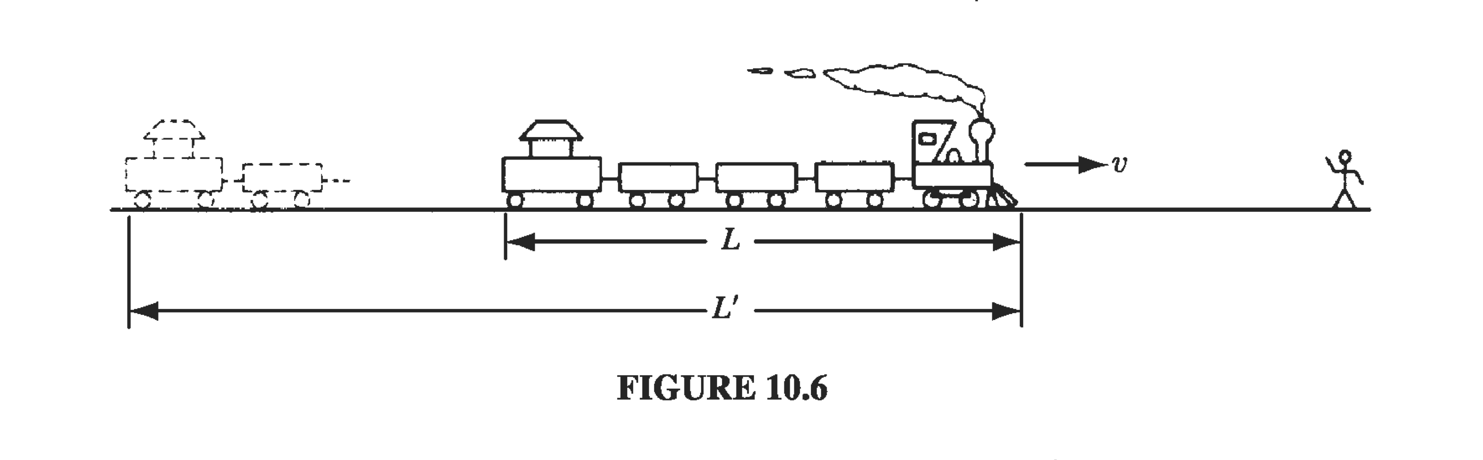
This is a purely geometrical effect, and it may help to tell the story in a less abstract context. You will not have noticed it, for obvious reasons, the the fact is that a train coming towards you looks a little longer than it really is, because the light you receive from the caboose left earlier than the light you receive simultaneously from the engine, and at that earlier time the train was farther away (Fig 10.6). In the interval it takes light from the caboose to travel the extra distance \( L’ \), the train itself moves a distance \( L’ - L \)
\[\frac{L'}{c} = \frac{L' - L}{v} \quad \text{or} \quad L' = \frac{L}{1-v/c} \]
So approaching trains appear longer, by a factor \( (1 - v/c)^{-1} \). By contrast, a train going away from you looks shorter, by a factor \( (1 + v/c)^{-1} \). In general, if the train’s velocity makes an angle \( \theta \) with your line of sight, the extra distance light from the caboose must cover is \( L’ \cos \theta \). In the time \( L’ \cos \theta / c \), then, the train moves a distance \( (L’ - L) \)
\[\frac{L' \cos \theta}{c} = \frac{L' - L}{v} \quad \text{or} \quad L' = \frac{L}{1 - v \cos \theta / c} \]Since the effect does not distort the dimensions perpendicular to the motion, we can easily move to 3D as
\[L' = \frac{l}{1 - \vu \gr \cdot \vec v / c} \]and the apparent volume of the train \( \tau’ \) of the train is then related to the actual volume by
\[\tau' = \frac{\tau}{1 - \vu \gr \cdot \vec v / c} \]where \( \vu \gr \) is a unit vector from the train to the observer.
Back to our moving point charge, the retarded time is determined implicitly by
\[| \vec r - \vec w(t_r)| = c(t - t_r)\] \[\vec \gr = \vec r - \vec w(t_r)\]It follows that
\[V( \vec r, t) = \frac{1}{4 \pi \epsilon_0} \frac{qc}{(\gr c - \vec \gr \cdot \vec v)}\]where \( \vec v \) is the velocity of the charge at the retarded time, and \( \vec \gr \) is the vector from the retarded position to the field point \( \vec r \). Moreover, since the current density is \( \rho \vec v \), the vector potential is
\[\begin{aligned} \vec A ( \vec r, t) & = & \frac{\mu_0}{4 \pi} \int \frac{\rho(\vec r', t_r) \vec v(t_r)}{\gr} \dd \tau' \\ & = & \frac{\mu_0}{4 \pi} \frac{\vec v}{\gr} \int \rho(\vec r', t_r) \dd \tau' \\ & = & \frac{\mu_0}{4 \pi} \frac{qc \vec v}{(\gr c - \vec \gr \cdot \vec v)} \\ & = & \frac{\vec v}{c^2} V(\vec r, t) \end{aligned}\]These are the Lienard-Wiechert potentials for a moving point charge.
10.3.2: The Fields of a Moving Point Charge#
After a great deal of vector calculus, starting from the Lienard-Wiechert potentials for a moving point charge, you can work out the fields
\[\vec E = - \grad V - \pdv{\vec{A}}{t} \qquad \vec B = \curl \vec A\]Because of all the various dependencies on \( \vec r, \vec r’, \vec \gr \), the integration is tricky, but eventually the result is
\[\vec E(\vec r, t) = \frac{q}{4 \pi \epsilon_0} \frac{ \gr}{(\vec \gr \cdot \vec u)^3} \left[ (c^2 - v^2) \vec u + \gr \cross ( \vec u \cross \vec a) \right]\]where we introduce the vector
\[\vec u \equiv c \vu \gr - \vec v\]and \( \vec a = \pdv{\vec v}{t} \) is the acceleration of the particle at the retarded time.