11.1 Dipole Radiation#
11.1.1 Electric Dipole Radiation#
Consider a dipole which is “oscillating” at some particular frequency. This looks like two metal spheres separated by distance \( d \) and connected by a small wire; at time \( t \) the charge on the upper sphere is \( q(t) \) and the charge on the lower sphere is \( -q(t) \). We drive the charge back and forth through the wire from one sphere to the other at an angular frequency \( \omega \)
\[q(t) = q_0 \cos (\omega t)\]The dipole moment is
\[\vec p(t) = p_0 \cos (\omega t) \vu z \qquad p_0 \equiv q_0 d\]Of course, we consider the harmonically oscillating dipole because we can build any other oscillations out of this basis.
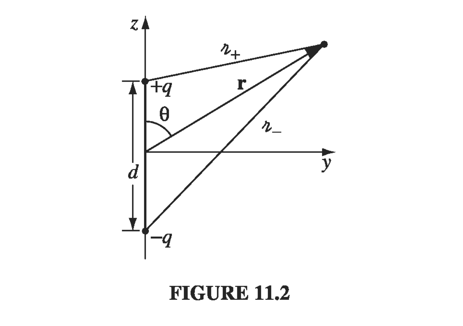
The retarded potential of this oscillating dipole is the superposition of the two point charges:
\[V(\vec r, t) = \frac{1}{4 \pi \epsilon_0} \left[ \frac{q_0 \cos [\omega(t - \gr_+ / c)]}{\gr_+} - \frac{q_0 \cos[\omega(t - \gr_- / c)]}{\gr_-} \right]\]where
\[\gr_{\pm} = \sqrt{ r^2 \mp r d \cos \theta + (d/2)^2}\]To take this physical dipole towards a perfect dipole, we want
\[d \ll r \quad \text{ while } \quad q_0 d = \text{const.}\]This approximation gives us
\[\gr_{\pm} \approx r \left( 1 \mp \frac{d}{2r} \cos \theta \right)\]so that
\[\frac{1}{\gr_{\pm}} \approx \frac{1}{r} \left( 1 \pm \frac{d}{2r} \cos \theta \right)\]and
\[\begin{aligned} \cos[\omega(t - \gr_{\pm} / c)] & \approx \cos \left[ \omega(t - r/c) \pm \frac{\omega d}{2c} \cos \theta \right] \\ & = \cos [ \omega(t - r/c)] \cos \left( \frac{\omega d}{2c} \cos \theta \right) \\ & \quad \pm \sin[\omega(t - r/c)] \sin \left( \frac{\omega d}{2c} \cos \theta \right) \end{aligned}\]In the limit of a perfect dipole, we take the dipole approximation
\[d \ll \frac{c}{\omega}\]Under that condition,
\[\cos [ \omega(t - \gr_{\pm}/c)] \approx \cos [\omega(t - r/c)] \mp \frac{\omega d}{2c} \cos \theta \sin [\omega(t - r/c)]\]Finally, we do not really care what happens near the origin. Rather, we are looking for the far-field behavior of the radiation, so we must consider fields that survive at large distances from the source:
\[r \gg \frac{c}{\omega}\]In this region, the retarded potential reduces to
\[V(r, \theta, t) = - \frac{p_0 \omega}{4 \pi \epsilon_0 c} \left( \frac{\cos \theta}{r} \right) \sin [ \omega(t - r/ c)]\]What about the vector potential? In our model of spheres connected by a wire, it is determined by the current flowing in the wire:
\[\vec I(t) = \dv{q}{t} \vu z = - q_0 \omega \sin(\omega t) \vu z\]so
\[\begin{aligned} \vec A & = & \frac{\mu_0}{4 \pi} \int \frac{ \vec J(\vec r', t_r)}{\gr} \dd \tau' \\ & = & \frac{\mu_0}{4 \pi} \int_{-d/2} ^{d/2} \frac{- q_0 \omega \sin [ \omega(t - \gr / c)]\vu z}{\gr} \dd z \end{aligned}\]Given our previous approximations, since the integration itself happens over the assumed short distance \( d \), we can replace the integrand by its value at the center and introduce a factor of \( d \)
\[\vec A(r, \theta, t) = - \frac{\mu_0 p_0 \omega}{4 \pi r} \sin [\omega(t - r/c)] \vu z\]Great, we’ve got the potentials! What are the fields in the radiation zone (far-field)?
\[\begin{aligned} \grad V & = & \pdv{V}{r} \vu r + \frac{1}{r} \pdv{V}{\theta} \vu \theta \\ & = & - \frac{p_0 \omega}{4 \pi \epsilon_0 c} \left[ \cos \theta \left( - \frac{1}{r^2} \sin [\omega (t - r/c)] - \frac{\omega}{rc} \cos [\omega(t - r/c)] \right) \vu r \right. \\ & & \qquad \left. - \frac{\sin \theta}{r^2} \sin [\omega(t - r/c)] \vu \theta \right] \\ & \approx & \frac{p_0 \omega^2}{4 \pi \epsilon_0 c^2} \left( \frac{\cos \theta}{r} \right) \cos [\omega(t - r/c)] \vu r \end{aligned}\]where we’ve dropped the first and last terms in accordance with our far-field approximation. Similarly,
\[\pdv{\vec A}{t} = - \frac{\mu_0 p_0 \omega^2}{4 \pi r} \cos [\omega(t - r/c)] (\cos \theta \vu r - \sin \theta \vu \theta)\]therefore
\[\vec E = - \grad V - \pdv{\vec A}{t} = - \frac{\mu_0 p_0 \omega^2}{4 \pi} \left( \frac{\sin \theta}{r} \right) \cos [ \omega( t - r/c)] \vu \theta\]What about the magnetic field?
\[\curl \vec A = \frac{1}{r} \left[ \pdv{}{r} (r A_\theta) - \pdv{A_r}{\theta} \right] \vu \phi \\ = - \frac{\mu_0 p_0 \omega}{4 \pi r} \left[ \sin \theta \cos [ \omega(t - r/c)] + \frac{\sin \theta}{r} [\omega(t - r/c)] \right] \vu \phi\]The second term can be eliminated in the far-field, so
\[\vec B = \curl \vec A = - \frac{\mu_0 p_0 \omega^2}{4 \pi c} \left( \frac{\sin \theta}{r} \right) \cos [\omega(t - r/c)]\vu \phi\]These fields are in phase, mutually perpendicular, and transverse to the direction of propagation, and the ratio of their amplitudes is \( E_0 / B_0 = c \), exactly as we expect from electromagnetic waves. These are actually spherical waves, not plane waves, and their amplitude decreases like \( 1/r \) as they progress. But for large r, they are approximately plane over small regions.
The energy flux is determined by the Poynting vector
\[\vec S(\vec r, t) = \frac{1}{\mu_0} \vec E \cross \vec B = \frac{\mu_0}{c} \left[ \frac{p_0 \omega^2}{4 \pi} \left( \frac{\sin \theta}{r} \right) \cos [\omega(t - r/c)] \right]^2 \vu r\]The intensity is the time average over a cycle
\[I = \langle \vec S \rangle = \left( \frac{\mu_0 p_0 ^2 \omega^4}{32 \pi^2 c} \right) \frac{\sin^2 \theta}{r^2} \vu r\]and the total power radiated is found by integrating \( \langle \vec S \rangle \) over a sphere of radius \( r \):
\[\langle P \rangle = \int \langle \vec S \rangle \cdot \dd \vec a = \frac{\mu_0 p_0 ^2 \omega^4}{32 \pi^2 c} \int \frac{\sin^2 \theta}{r^2} r^2 \sin \theta \dd \theta \dd \phi = \frac{\mu_0 p_0 ^2 \omega^4}{12 \pi c} \]