2.4: Work and Energy in Electrostatics#
2.4.1: The Work it Takes to Move a Charge#
Suppose you have a stationary configuration of source charges, and you want to move a test charge Q from point a to point b (Fig. 2.39). Question: how much work will you have to do? At any point along the path, the electric force on Q is \( \vec{F} = Q \vec{E} \); the force you must exert, in opposition to the electric force, is \( -Q\vec{E} \). The work you do is therefore
\[W = \int_{a}^{b} \vec{F} \cdot \dd{\vec{l}} \\ = - Q \int_{a}^{b} \vec{E} \cdot \dd{\vec{l}} \\ = - Q[V(b) - V(a)]\]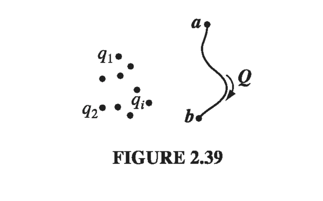
Notice that the answer is independent of the path you take from a to b; in mechanics, then, we would call the electrostatic force “conservative.” Dividing through by Q, we have
\[V(b) - V(a) = \frac{W}{Q} \]In words, the potential difference between points a and b is equal to the work per unit charge required to carry a particle from a to b. In particular, if you want to bring Q in from far away and stick it at point r, the work you must do is
\[W = Q[V(\vec{r}) - V(\infty)],\]so if you have set the reference point at infinity,
\[W = Q V(\vec{r}) \label{2.39} \tag{2.39}\]In this sense, potential is potential energy (the work it takes to create a system) per unit charge (just as the field is force per unit charge).
2.4.2: The Energy of a Point Charge Distribution#
How much work would it take to assemble an entire collection of point charges? Imagine bringing in the charges, one by one, from far away (Fig 2.40). The first charge \( q_1 \) takes no work, since there is no field to fight against. Now bring in \( q_2 \). According to \( \eqref{2.39} \) this will cost you \( q_2 V_1(\vec{r}_2) \), where \( V_1 \) is the potential due to \( q_1 \) , and \( \vec{r}_2 \) is the place we’re putting \( q_2 \):
\[W_2 = \frac{1}{4 \pi \epsilon_0} q_2 \left( \frac{q_1}{\gr_{12}} \right)\](\( \gr_{12} \) is the distance between \( q_1 \) and \( q_2 \), once they are in position). As you bring in each charge, nail it down in its final location, so it doesn’t move when you bring in the next charge. Now bring in \( q_3 \). This requires work \( q_3 V_{1,2}(\vec{r}3) \), where \( V{1,2} \) is the potential due to charges \( q_1 \) and \( q_2 \), namely \( (1 / 4 \pi \epsilon_0) (q_1 / \gr_{13} + q_2 / \gr_{23} ) \). Thus
\[W_3 = \frac{1}{4 \pi \epsilon_0} q_3 \left( \frac{q_1}{\gr_{13}} + \frac{q_2}{\gr_{23}} \right)\]Similarly, the extra work to bring in \( q_4 \) will be
\[W_4 = \frac{1}{4 \pi \epsilon_0} q_4 \left( \frac{q_1}{\gr_{14}} + \frac{q_2}{\gr_{24}} + \frac{q_3}{\gr_{34}} \right)\]The total work necessary to assemble the first four charges, then, is
\[W = \frac{1}{4 \pi \epsilon_0} \left( \frac{q_1 q_2}{\gr_{12}} + \frac{q_1 q_3}{\gr_{13}} + \frac{q_1 q_4}{\gr_{14}} + \frac{q_2 q_3}{\gr_{23}} + \frac{q_2 q_4}{\gr_{24}} + \frac{q_3 q_4}{\gr_{34}} \right)\]You see the general rule: Take the product of each pair of charges, divide by their separation distance, and add it all up:
\[W = \frac{1}{4 \pi \epsilon_0} \sum_{i = 1} ^{n} \sum_{j > i} ^n \frac{q_i q_j}{\gr_{ij}} \]The stipulation \( j > i \) is to remind you not to count the same pair twice. A nicer way to accomplish this is intentionally to count each pair twice, and then divide by 2:
\[W = \frac{1}{8 \pi \epsilon_0} \sum_{i = 1} ^n \sum_{j \neq i} \frac{q_i q_j}{\gr_{ij}} \](we must still avoid \( i = j \), of course). Notice that in this form the answer plainly does not depend on the order in which you assemble the charges, since every pair occurs in the sum.
Finally, let’s pull out the factor \( q_i \):
\[W = \frac{1}{2} \sum_{i = 1}^n q_i \left( \sum_{j \neq i} ^n \frac{1}{4 \pi \epsilon_0} \frac{q_j}{\gr_{ij}} \right)\]The term in parentheses is the potential at point \( \vec{r_i} \) (the position of \( q_i \) ) due to all the other charges - all of them, now, not just the ones that were present at some stage during the assembly. Thus,
\[W = \frac{1}{2} \sum_{i = 1} ^n q_i V(\vec{r_i}) \label{2.42} \tag{2.42}\]That’s how much work it takes to assemble a configuration of point charges; it’s also the amount of work you’d get back if you dismantled the system. In the meantime, it represents energy stored in the configuration (“potential” energy, if you insist, though for obvious reasons I prefer to avoid that word in this context).
2.4.3: The Energy of a Continuous Charge Distribution#
For a volume charge density \( \rho \), \( \eqref{2.42} \) becomes
\[W = \frac{1}{2} \int \rho V \dd{\tau} \label{2.43} \tag{2.43}\]There is a lovely way to write this result, in which \( \rho \) and \( V \) are eliminated in favor of \( \vec{E} \). First, use Gauss’s law to express \( \rho \) in terms of \( \vec{E} \)
\[\rho = \epsilon_0 \div{\vec{E}} \qquad \text{so,} \qquad W = \frac{\epsilon_0}{2} \int (\div{\vec{E}}) V \dd{\tau}\]Now, use integration by parts to transfer the derivative from \( \vec{E} \) to \( V \):
\[W = \frac{\epsilon_0}{2} \left[ - \int \vec{E} \cdot (\grad{V}) \dd{\tau} + \oint V \vec{E} \cdot \dd{\vec{a}} \right]\]But \( \grad{V} = - \vec{E} \), so
\[ W = \frac{\epsilon_0}{2} \left( \int_{\mathscr{V}} E^2 \dd{\tau} + \oint V \vec{E} \cdot \dd{\vec{a}} \right) \label{2.44} \tag{2.44} \]But what volume is this we’re integrating over? Let’s go back to the formula we started with, \( \eqref{2.43} \). From its derivation, it is clear that we should integrate over the region where the charge is located. But actually, any larger volume would do just as well: The “extra” territory we throw in will contribute nothing to the integral, since \( \rho = 0 \) out there. With this in mind, we return to \( \eqref{2.44} \). What happens here, as we enlarge the volume beyond the minimum necessary to trap all the charge? Well, the integral of \( E^2 \) can only increase (the integrand being positive); evidently the surface integral must decrease accordingly to leave the sum intact. (In fact, at large distances from the charge, \( E \) goes like \( 1 / r^2 \) and \( V \) like \( 1/r \), while the surface area grows like \( r^2 \); roughly speaking, then, the surface integral goes down like \( 1/r \). Please understand: \( \eqref{2.44} \) gives you the correct energy W, whatever volume you use (as long as it encloses all the charge), but the contribution of the volume integral goes up, and that of the surface integral goes down, as you take larger and larger volumes. In particular, why not integrate over all space? Then the surface integral goes to zero, and we are left with
\[W = \frac{\epsilon_0}{2} \int E^2 \dd{\tau} \quad \text{(all space)} \label{2.45} \tag{2.45}\]Example 2.9#
Find the energy of a uniformly charged spherical shell of total charge \( q \) and radius \( R \)
Use \( \eqref{2.43} \) in the version appropriate to surface charges
\[W = \frac{1}{2} \sigma V \dd{a}\]Now, the potential at the surface of this sphere is \( (1/4 \pi \epsilon_0)q/R \) (a constant), so
\[W = \frac{1}{8\pi \epsilon_0} \frac{q}{R} \int \sigma \dd{a} = \frac{1}{8 \pi \epsilon_0} \frac{q^2}{R} \]Solution 2 Use \( \eqref{2.45} \). Inside the sphere, \( \vec{E} = 0 \); outside:
\[\vec{E} = \frac{1}{4\pi \epsilon_0} \frac{q}{r^2} \vu{r} \quad \text{so} \quad E^2 = \frac{q^2}{(4 \pi \epsilon_0)^2 r^4} \]Therefore,
\[W_{tot} = \frac{\epsilon_0}{2 (4 \pi \epsilon_0)^2}\int \left( \frac{q^2}{r^4} \right) (r^2 \sin \theta \dd{r} \dd{\theta} \dd{\phi}) \\ = \frac{1}{32 \pi ^2 \epsilon_0} q^2 4 \pi \int_{R} ^{\infty} \frac{1}{r^2} \dd{r} = \frac{1}{8 \pi \epsilon_0} \frac{q^2}{R} \]2.4.4: Comments on Electrostatic Energy#
A perplexing “inconsistency”
Equation \( \eqref{2.45} \) clearly implies that the energy of a stationary charge distribution is always positive. On the other hand, \( \eqref{2.42} \) (from which \( \eqref{2.45} \) was in fact derived), can be positive or negative. For instance, according to \( \eqref{2.42} \) the energy of two equal but opposite charges a distance \( \gr \) apart is \( -(1/4 \pi \epsilon_0) (q^2/\gr) \). What’s gone wrong? Which equation is correct?
The answer is that both are correct, but they speak to slightly different questions. Equation \( \eqref{2.42} \) does not take into account the work necessary to make the point charges in the first place; we started with point charges and simply found the work required to bring them together. This is wise strategy, since \( \eqref{2.45} \) indicates that the energy of a point charge is in fact infinite
\[ W = \frac{\epsilon_0}{2(4 \pi \epsilon_0)^2} \int \left( \frac{q^2}{r^4} \right) (r^2 \sin \theta \dd{r} \dd{\theta} \dd{\phi}) = \frac{q^2}{8 \pi \epsilon_0} \int_{0} ^{\infty} \frac{1}{r^2} \dd{r} = \infty \]Equation \( \eqref{2.45} \) is more complete, in the sense that it tells you the total energy stored in a charge configuration, but \( \eqref{2.42} \) is more appropriate when you’re dealing with point charges, because we prefer (for good reason!) to leave out that portion of the total energy that is attributable to the fabrication of the point charges themselves. In practice, after all, the point charges (electrons, say) are given to us ready-made; all we do is move them around. Since we did not put them together, and we cannot take them apart, it is immaterial how much work the process would involve. (Still, the infinite energy of a point charge is a recurring source of embarrassment for electromagnetic theory, afflicting the quantum version as well as the classical. We shall return to the problem in Chapter 11).
Now, you may wonder where the inconsistency crept into an apparently water-tight derivation. The “flaw” lies between \( \eqref{2.42} \) and \( \eqref{2.43} \): in the former, \( V(\vec{r_i}) \) represents the potential due to all the other charges, but not \( q_i \), whereas in the latter, \( V(\vec{r}) \) is the full potential. For a continuous distribution, there is no distinction, since the amount of charge right at the point \( \vec{r} \) is vanishingly small, and its contribution to the potential is zero. But in the presence of point charges you’d better stick with \( \eqref{2.42} \).
Where is the energy stored? Equations \( \eqref{2.43} \) and \( \eqref{2.45} \) offer two different ways of calculating the same thing. The first is an integral over the charge distribution, the second is an integral over the field. These can involve completely different regions. For instance, in the case of a spherical shell, the charge is confined to the surface, whereas the electric field is everywhere outside this surface. Where is the energy, then? Is it stored in the field, as \( \eqref{2.45} \) seems to suggest, or is it stored in the charge, as \( \eqref{2.43} \) implies? At the present stage this is simply an unanswerable question: I can tell you what the total energy is, and I can provide you with several different ways to compute it, but it is impertinent to worry about where the energy is located. In the context of radiation theory (Chapter 11) it is useful (and in general relativity it is essential) to regard the energy as stored in the field, with a density
\[\frac{\epsilon_0}{2} E^2 = \text{ energy per unit volume} \label{2.46} \tag{2.46}\]But in electrostatics one could just as well say it is stored in the charge, with a density \( \frac{1}{2} \rho V \). The difference is purely a matter of bookkeeping.
The superposition principle. Because electrostatic energy is quadratic in the fields, it does not obey a superposition principle. The energy of a compound system is not the sum of the energies of its parts considered separately - there are also “cross terms”:
\[\begin{aligned} W_{tot} & = & \frac{\epsilon_0}{2} \int E^2 \dd{\tau} = \frac{\epsilon_0}{2} \int (\vec{E_1} + \vec{E_2})^2 \dd{\tau} \\ & = & \frac{\epsilon_0}{2} \int (E_1 ^2 + E_2 ^2 + 2 \vec{E_1} \cdot \vec{E_2}) \dd{\tau} \\ & = & W_1 + W_2 + \epsilon_0 \int \vec{E_1} \cdot \vec{E_2} \dd{\tau} \end{aligned}\]For example, if you double the charge everywhere, you quadruple the total energy.