6.2: The Field of a Magnetized Object#
6.2.1: Bound Currents#
Suppose we have a piece of magnetized material; the magnetic dipole moment per unit volume, M, is given. What field does this object produce? Well, the vector potential of a single dipole m is given by Eq. 5.85
\[\vec{A}_{dip} (r) = \frac{\mu_0}{4 \pi} \frac{\vec{m} \cross \vu{r}}{r^2}\]In the magnetized object, each volume element \( \dd \tau’ \) carries a dipole moment \( M \dd \tau’ \), so the total vector potential is (Fig 6.11)
\[\vec{A}(r) = \frac{\mu_0}{4 \pi} \int \frac{\vec{M}(r') \cross \vu{\gr}}{\gr ^2} \dd \tau' \tagl{6.11}\]That does it, in principle. But, as in the electrical case, the integral can be cast in a more illuminating form by exploiting the identity
\[\grad ' \frac{1}{\gr} = \frac{\vu{\gr}}{\gr^2} \]With this,
\[\vec{A}(r) = \frac{\mu_0}{4 \pi} \int \left[ \vec{M}(r') \cross \left( \grad ' \frac{1}{\gr} \right) \right] \dd \tau'\]Integrating by parts gives
\[\vec{A}(r) = \frac{\mu_0}{4 \pi} \left( \int \frac{1}{\gr} [ \grad ' \cross \vec{M}(r') ] \dd \tau' - \int \grad' \cross \left[ \frac{\vec{M}(r')}{\gr} \right] \dd \tau' \right)\]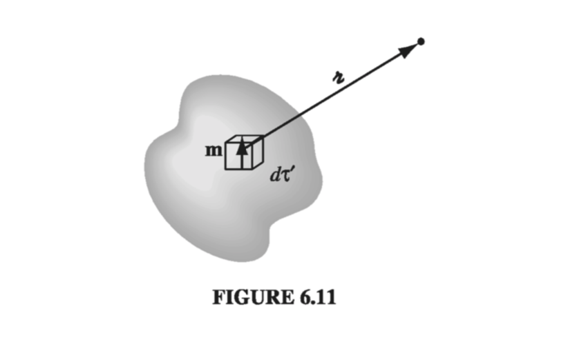
The first term looks just like the potential of a volume current
\[\vec{J}_b = \curl \vec{M} \tagl{6.13}\]while the second looks like the potential of a surface current
\[\vec{K_b} = \vec{M} \cross \vu{n} \tagl{6.14}\]where \( \vu{n} \) is the normal unit vector. With these definitions,
\[\vec{A}(r) = \frac{\mu_0}{4\pi} \int_V \frac{\vec{J_b}(r')}{\gr} \dd \tau' + \frac{\mu_0}{4 \pi} \oint _S \frac{\vec{K_b}(r')}{\gr} \dd a' \tagl{6.15}\]What this means is that the potential (and hence also the field) of a magnetized object is the same as would be produced by a volume current \( \vec{J_b} = \curl \vec{M} \) throughout the material, plus a surface current \( \vec{K_b} = \vec{M} \cross \vu{n} \), on the boundary. Instead of integrating the contributions of all the infinitesimal dipoles, using Eq. 6.11, we first determine the bound currents, and then find the field they produce, in the same way we would calculate the field of any other volume and surface currents. Notice the striking parallel with the electrical case: there the field of a polarized object was the same as that of a bound volume charge \( \rho_b = - \div \vec{P} \) plus a bound surface charge \( \sigma_b = \vec{P} \cdot \vu{n} \).
Example 6.1#
Find the magnetic field of a uniformly magnetized sphere
Choosing the z axis along the direction of M (Fig 6.12), we have
\[\vec{J}_b = \curl \vec{M} = 0, \qquad \vec{K}_b = \vec{M} \cross \vu{n} = M \sin \theta \vu{\phi}\]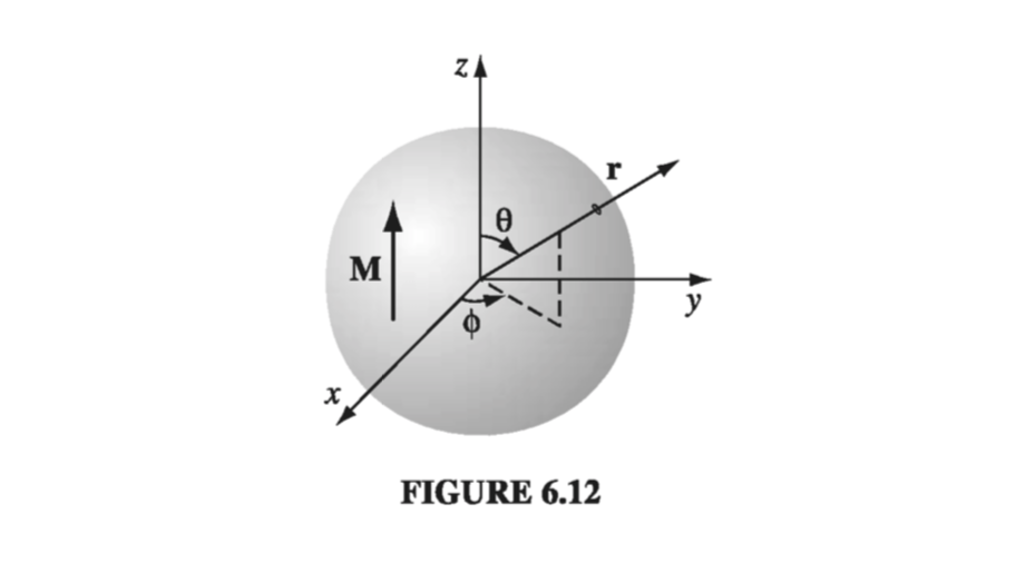
which we already worked out in Exercise 5.11. So, identifying \( \sigma R \vec{\omega} \rightarrow \vec{M} \), we can write down
\[\vec{B} = \frac{2}{3} \mu_0 \vec{M} \tagl{6.16}\]inside the sphere, and outside the sphere the field is that of a perfect dipole
\[\vec{m} = \frac{4}{3} \pi R^3 \vec{M}\] \[\rightarrow \quad \vec{B} = \frac{4 \mu_0 R^3}{9 r^3} (2 \cos \theta \vu{r} + \sin \theta \vu{\theta} )\]Notice that the internal field is uniform, like the electric field inside a uniformly polarized sphere (Eq. 4.14), although the actual formulas for the two cases are curiously different ( \( \frac{2}{3} \) in place of \( -\frac{1}{3} \)). The external fields are also analogous: pure dipole in both instances.
6.2.2: Physical Interpretation of Bound Currents#
In the last section, we found that the field of a magnetized object is identical to the field that would be produced by a certain distribution of “bound” currents, \( \vec{J}_b \) and \( \vec{K}_b \). I want to show you how these bound currents arise physically. This will be a heuristic argument - the rigorous derivation has already been given. Figure 6.15 depicts a thin slab of uniformly magnetized material, with the dipoles represented by tiny current loops. Notice that all the “internal” currents cancel: every time there is one going to the right, a contiguous one is going to the left. However, at the edge there is no adjacent loop to do the canceling. The whole thing, then, is equivalent to a single ribbon of current I flowing around the boundary (Fig. 6.16).
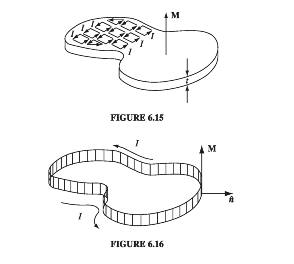
What is this current, in terms of M? Say that each of the tiny loops has area a and thickness t (Fig 6.17). In terms of the magnetization, its dipole moment is \( m = M a t \). In terms of the circulating current I, however, \( m = I a \). Therefore \( I = M t \), so the surface current is \( K_b = I / t = M \). Using the outward-drawn unit vector \( \vu{n} \) (Fig 6.16), the direction of \( \vec{K_b} \) is conveniently indicated by the cross product:
\[\vec{K_b} = \vec{M} \cross \vu{n}\](This expression also records the fact that there is no current on the top or bottom surface of the slab; here M is parallel to \( \vu{n} \), so the cross product vanishes.)
This bound surface current is exactly what we obtained in Sect. 6.2.1. It is a peculiar kind of current, in the sense that no single charge makes the whole trip - on the contrary, each charge moves only in a tiny little loop within a single atom. Nevertheless, the net effect is a macroscopic current flowing over the surface of the magnetized object. We call it a “bound” current to remind ourselves that every charge is attached to a particular atom, but it’s a perfectly genuine current, and it produces a magnetic field in the same way any other current does.
When the magnetization is nonuniform, the internal currents no longer cancel. Figure 6.18(a) shows two adjacent chunks of magnetized material, with a larger arrow on the one to the right suggesting greater magnetization at that point. On the surface where they join, there is a net current in the x direction, given by
\[I_x = [M_z (y + \dd y) - M_z (y)] \dd z = \pdv{M_z}{y} \dd y \dd z\]The corresponding volume current density is therefore
\[(J_b)_x = \pdv{M_z}{y}\]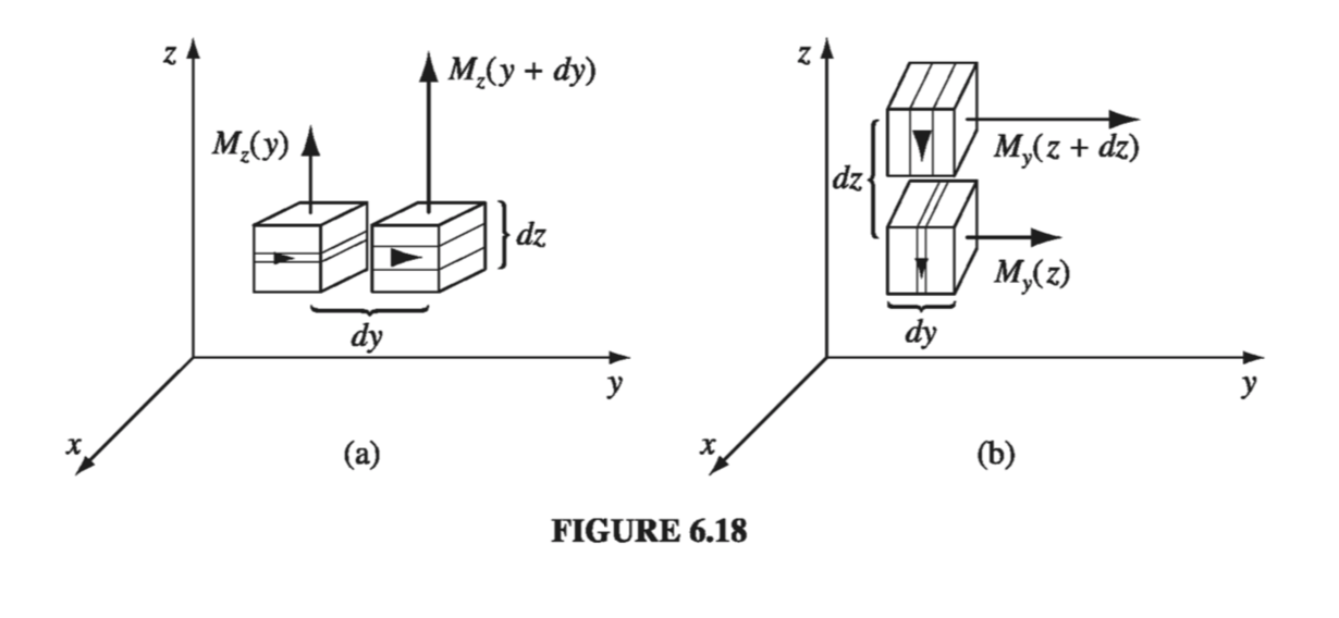
By the same token, a nonuniform magnetization in the y direction would contribute an amount
\[(J_b)_x = \pdv{M_z}{y} - \pdv{M_y}{z}\]In general, then
\[\vec{J_b} = \curl \vec{M}\]consistent, again, with the result of Section 6.2.1.
Incidentally, like any other steady current, \( \vec{J_b} \) should obey the conservation law 5.33
\[\div \vec{J_b} = 0\]Does it? Yes, for the divergence of a curl is always zero.
6.2.3: The Magnetic Field Inside Matter#
Like the electric field, the actual microscopic magnetic field inside matter fluctuates wildly from point to point and instant to instant. When we speak of “the” magnetic field in matter, we mean the macroscopic field: the average over regions large enough to contain many atoms. (The magnetization M is “smoothed out” in the same sense.) It is this macroscopic field that one obtains when the methods of Sect. 6.2.1 are applied to points inside magnetized material, as you can prove for yourself in the following problem.
Problem 6.11#
In Sect 6.2.1, we began with the potential of a perfect dipole (Eq. 6.10), whereas in fact we are dealing with physical dipoles. Show, by the method of Section 4.2.3, that we nonetheless get the correct macroscopic field.
As in Section 4.2.3, we want the average of
\[\vec{B} = \vec{B} _{out} + \vec{B}_{in}\]where \( \vec{B} _ {out} \) is due to molecules outside a small sphere around point P, and \( \vec{B} _ {in} \) is due to molecules inside the sphere. The average of \( \vec{B} _ {out} \) is the same as the field at the center, and for this it is OK to use Equation 6.10, since the center is “far” from all the molecules in question:
\[\vec{A}_{out} = \frac{\mu_0}{4 \pi} \int_{outside} \frac{\vec{M} \cross \vu{\gr}}{\gr ^2} \dd \tau \]The average of \( \vec{B} _ {in} \) is \( \frac{\mu_0}{4 \pi} \frac{2 \vec{m}}{R^3} \) - Equation 5.93 - where \( \vec{m} = \frac{4}{3} \pi R^3 \vec{M} \). Thus the average \( \vec{B} _ {in} \) is \( 2 \mu_0 \vec{M}/3 \). But what is left out of the integral \( \vec{A} _ {out} \) is the contribution of a uniformly magnetized sphere, to wit \( 2 \mu_0 \vec{M} / 3 \) (Equation 6.16), and this is precisely what \( \vec{B}_{in} \) puts back in. So we’ll get the correct macroscopic field using Equation 6.10.