9.1: Electromagnetic Waves in One Dimension#
9.1.1 THE WAVE EQUATION#
Before we start writing down how electromagnetic energy propagates in space as radiation, we’ll dust off our mathematical background on waves. Thanks to Fourier analysis, we know that sinusoidal waves form a complete basis for all periodic functions, so we restrict our investigation to sinusoidal variations.
Suppose some quantity “\( f \)” is propagating with speed \( v \) in the \( +z \) direction, and we focus on sinusoidal “disturbances.” At \( t = 0 \),
\[f = f_m \cos k z \qquad k = \frac{2 \pi}{\lambda}\]And at any time \( t = t \)
\[f = f_m \cos [ k ( z - vt) ] \] \[= a_m \cos ( kz - \omega t) \qquad \omega \equiv v k\]And if we look at a particular position \( z = 0 \) (or other) and watch \( f \) as a function of time, we’ll see the same sinusoidal behavior
\[f(z = 0, t) = f_m ( \omega t)\]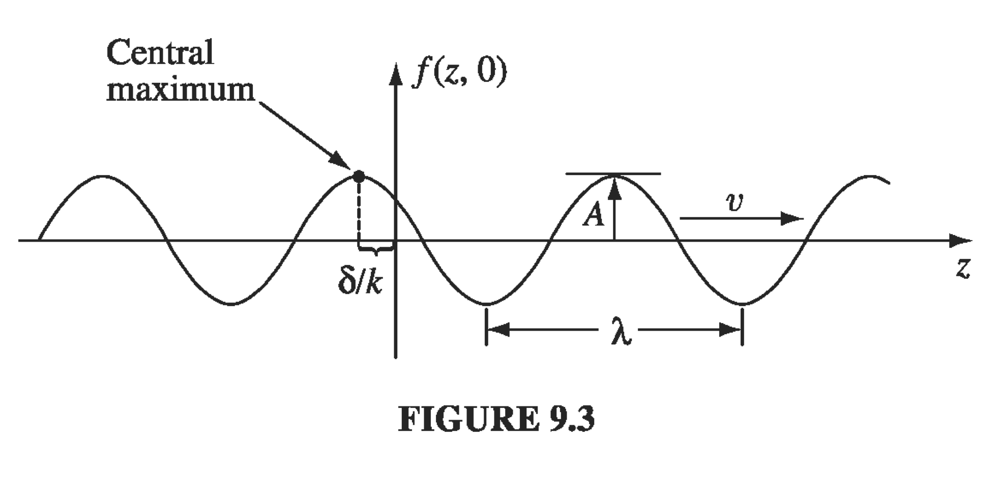
Generalizing to the 3-D case, instead of a wavenumber we have a wave vector \( \vec k = k_x \vu x + k_y \vu y + k_z \vu z \)
\[f = f_m \cos (\vec k \cdot \vec r - \omega t + \delta)\]Any wave that looks like this satisfies the wave equation
\[\frac{\partial ^2 a}{\partial z^2} = \frac{1}{v} \frac{\partial ^2 a}{\partial t^2} \qquad v = \frac{\omega}{k} \quad \text{(in 1-D)}\]