9.2.1 Wave Equation for E and B#
Recall Maxwell’s equations
\[\begin{aligned} (\text{i}) & \quad \div \vec{D} = \rho_f \quad \text{(Gauss's law)} \\ (\text{ii}) & \quad \div \vec{B} = 0 \quad \text{(Ng's Law)} \\ (\text{iii}) & \quad \curl \vec{E} = - \pdv{\vec{B}}{t} \quad \text{(Faraday's Law}) \\ (\text{iv}) & \quad \curl \vec{H} = \vec{J}_f + \pdv{\vec{D}}{t} \quad \text{(Ampere's Law)} \end{aligned}\]To get to a wave equation from these, we start with a curl of curl and use a standard vector identity
\[\curl (\curl \vec E) = \grad ( \div \vec E) - \grad ^2 \vec E\]Use Faraday’s law on the left hand side (and move the spatial derivative through the temporal one), and on the right hand side use Gauss’ law to re-write the divergence
\[\rightarrow - \pdv{}{t} ( \curl \vec B) = \frac{1}{\epsilon_0} \grad \rho - \grad ^2 \vec E\] \[\rightarrow - \pdv{}{t} \left( \mu_0 \vec J + \mu_0 \epsilon_0 \pdv{\vec{E}}{t} \right) = - \mu_0 \pdv{\vec J}{t} - \mu_0 \epsilon_0 \frac{\partial ^2 \vec E}{\partial t ^2} = \frac{\grad \rho}{\epsilon_0} - \grad ^2 \vec E\] \[\rightarrow \grad ^2 \vec E - \mu_0 \epsilon_0 \frac{\partial ^2 \vec E}{\partial t^2} = \frac{1}{\epsilon_0} \grad \rho + \mu_0 \pdv{\vec{J}}{t} \quad \text{"non-homogeneous" wave equation for E}\]In a vacuum, \( \rho = 0 \) and \( \vec J = 0 \) so
\[\grad ^2 \vec E - \mu_0 \epsilon_0 \frac{\partial ^2 \vec E}{\partial t^2} = 0\]which is just a standard 3D wave equation. We can identify the speed of propagation based on the constant of proportionality \( v = \frac{1}{\sqrt{\mu_0 \epsilon_0}} = c \)
We could also have started with \( \curl (\curl \vec B) \) to obtain
\[\grad ^2 \vec B - \mu_0 \epsilon_0 \frac{\partial ^2 \vec B}{\partial t^2} = - \mu_0 (\curl \vec J) \quad \text{"non-homogeneous" wave equation for B}\]So, in vacuum you get the exact same wave equation
\[\grad ^2 \vec B - \mu_0 \epsilon_0 \frac{\partial ^2 \vec B}{\partial t^2} = 0\]So, both \( \vec E \) and \( \vec B \) must satisfy these wave equations. We know that the wave equations admit certain sets of solutions, but that’s not the entire story. We’ll see additional constraints on solutions to \( \vec E \) and \( \vec B \) due to the fact that the waves need to satisfy all of the Maxwell equations, so \( \vec E \) and \( \vec B \) are very intimately linked.
9.2.2: Monochromatic Plane Waves#
Consider monochromatic sine waves (plane waves) in a single direction, so that all variation happens in the z-direction. Again, using the superposition principle we’ll be able to build up more complicated solutions.
\[\vec E = \vec E_0 \cos (k z - \omega t + \delta) \qquad \vec B = \vec B_0 \cos (k z - \omega t + \delta)\] \[\vec E_0 = E_{0, x} \vu x + E_{0, y} \vu y + E_{0, z} \vu z\]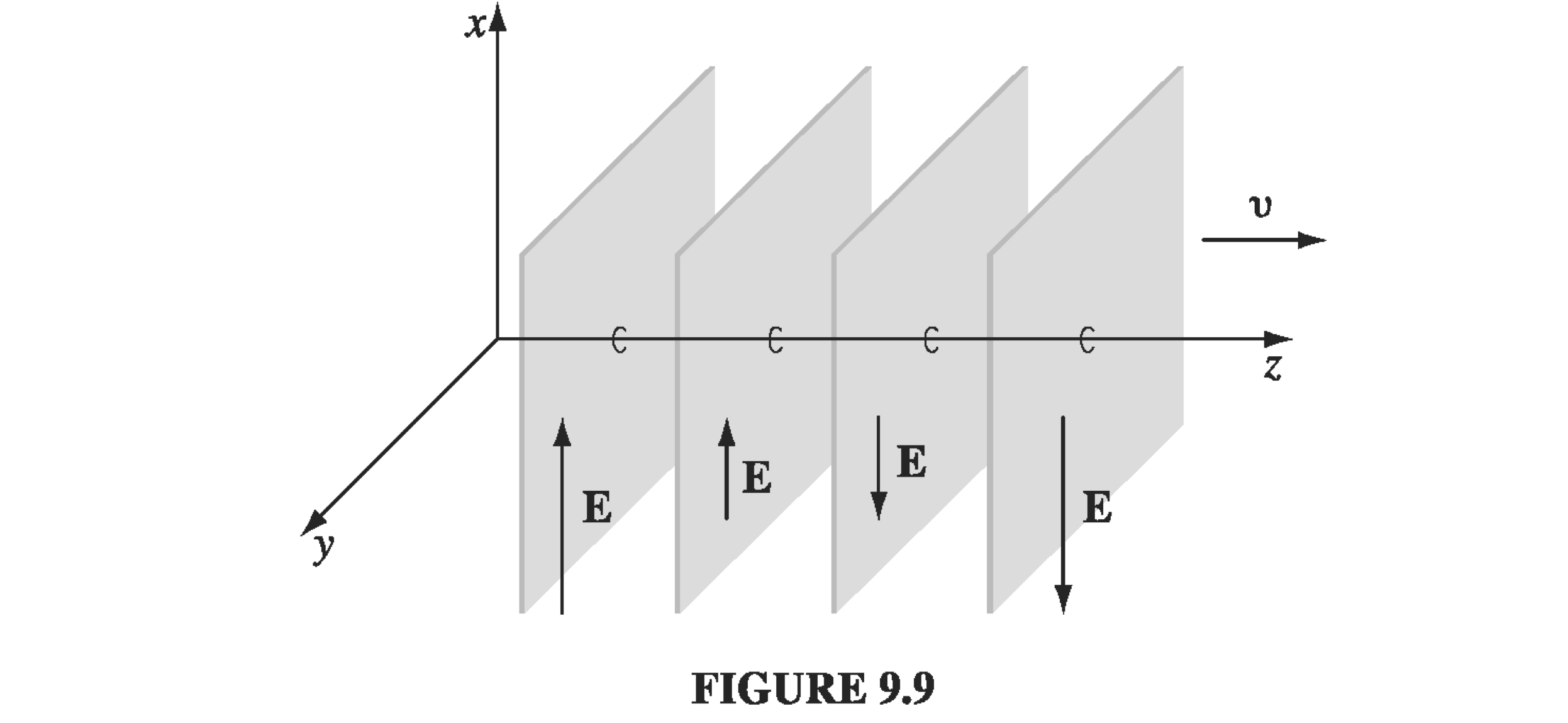
Let’s apply Gauss’ law (in vacuum)
\[\div \vec E = 0\] \[\div (\vec E_0 \cos (k z - \omega t + \delta) ) = 0\] \[\rightarrow \pdv{E_{0, x}}{x} \cos (k z - \omega t + \delta ) + \pdv{E_{0, y}}{y} \cos (kz - \omega t + \delta)\] \[+ \pdv{E_{0, z}}{z} \cos (kz - \omega t + \delta) + E_{0,z}(- k \sin(kt - \omega t + \delta)) = 0\]We’ve decided that there is no variation in the x- and y-directions, so only the final term survives, and must be equal to zero
\[E_{0, z} (- k \sin(kt - \omega t + \delta)) = 0 \quad \rightarrow \quad E_{0,z} = 0\]Which is to say that EM plane waves are “transverse” waves.
Let’s also use Faraday’s law to relate \( \vec E \) and \( \vec B \) :
\[\curl \vec E = - \pdv{B}{t}\] \[\curl \vec E = \begin{pmatrix} \vu x & \vu y & \vu z \\ \pdv{}{x} & \pdv{}{y} & \pdv{}{z} \\ E_{0, x} \cos (k z - \omega t) & E_{0, y} \cos (k z - \omega t) & 0 \end{pmatrix}\] \[= \vu x ( E_{0, y} k \sin(kz - \omega t)) - \vu y (E_{0, x} k \sin(k z - \omega t))\] \[- \pdv{B}{t} = - \vu x \pdv{}{t} B_{0, x} \cos (kz - \omega t) - \vu y \pdv{}{t}B_{0, y} \cos (kz - \omega t)\] \[= - \vu x B_{0, x} \omega \sin (k z - \omega t) - \vu y B_{0, y} \omega \sin (kz - \omega t)\]Matching up components and canceling the sine functions,
\[\rightarrow k E_{0, y} = - \omega B_{0, x} \qquad k E_{0, x} = \omega B_{0, y}\]So every time you have an \( \vec E \) field, you will have a \( \vec B \) field in an orthogonal direction - they are mutually orthogonal - and they are in phase, since the proportionality factors are real.
9.2.3: Energy and Momentum in Electromagnetic Waves#
To repeat, for monochromatic plane waves propagating in the z-direction,
\[\vec E = \vec{E_0} \cos ( k z - \omega t + \delta) = E_0 \cos (k z - \omega t + \delta) \vu x\] \[\vec B = B_0 \cos (kz - \omega t + \delta) \vu y\]and
\[E_0 / B_0 = c\]What does the energy density due to these fields look like?
\[u = \frac{1}{2} \epsilon_0 E^2 + \frac{1}{2\mu_0} B^2 = \epsilon_0 E^2 = \epsilon_0 E_0 \cos ^2 (kz - \omega t + \delta)\]The electric and magnetic contributions are equal. The resulting Poynting vector is
\[\vec S = \frac{1}{\mu_0} \vec E \cross \vec B = \frac{E_0 B_0 }{\mu_0} \cos ^2 (kz - \omega t + \delta ) \vu z\] \[= \frac{E_0 ^2}{\mu_0 c} \cos ^2 (kz - \omega t + \delta) \vu z = c \epsilon_0 E_0 ^2 \cos ^2 (kz - \omega t + \delta) \vu z\] \[\vec S = c u \vu z\]So the Poynting vector points in the direction of propagation, and it has amplitude \( c u \). What about the momentum density?
\[\vec g = \mu_0 \epsilon_0 \vec S = \epsilon_0 (\vec E \cross \vec B) = \frac{1}{c^2} cu \vu z = \frac{u}{c} \vu z\]The rate of oscillation of these waves is typically very high, so we are mostly interested in the average of the oscillatory behavior over a period. Recall that the time-average of \( \cos ^2 \) over a cycle is \( \frac{1}{2} \), so
\[\langle u \rangle = \frac{1}{2} \epsilon_0 E_0 ^2\] \[\langle \vec S \rangle = \frac{1}{2} c \epsilon_0 E_0 ^2 \vu z\] \[\langle \vec g \rangle = \frac{1}{2c} \epsilon_0 E_0 ^2 \vu z\]Another useful quantity we usually throw around is the Root Mean Square (RMS) value of the field
\[\sqrt{\langle E_0 ^2 \cos ^2 (kz - \omega t + \delta) \rangle } = \sqrt{\frac{E_0^2}{2}} = \frac{E_0}{\sqrt{2}} \approx 0.7 E_0\]The “intensity” of the electromagnetic wave is defined as its power per unit area, or energy per unit area per unit time
\[I = \frac{\text{power}}{\text{area}} = \frac{\text{energy}}{\text{area}\cdot\text{time}} \] \[= \langle | \vec S | \rangle = \langle | cu \vu z | \rangle = c \langle u \rangle = \frac{1}{2} c \epsilon_0 E_0 ^2\]If the light hits the surface of a perfect absorber, it will transfer its momentum to the surface. In a time \( \Delta t \) the momentum transfer will be
\[\Delta \vec p = \langle \vec g \rangle A c \Delta t\]so the radiation pressure (average force per unit area) is
\[P = \frac{1}{A} \frac{\Delta p}{\Delta t} = \frac{1}{2} \epsilon_0 E_0 ^2 = \frac{I}{c}\]Of course, when falling on a perfect reflector, the radiation pressure is twice as big, since the resulting momentum of the reflected light switches direction instead of being absorbed.
Example Problem 9.10#
The intensity of sunlight hitting the earth is about 1300 \( W/m^2 \). If sunlight strikes a perfect absorber, what pressure does it exert? How about a perfect reflector? What fraction of atmospheric pressure does this amount to?
The radiation pressure for a perfect absorber is
\[P = \frac{I}{c} = \frac{1300}{3 \cdot 10^8} \approx 4.3 \cdot 10^{-6} N/m^2\]The atmospheric pressure on earth’s surface is about \( 10^5 N \), so
\[\frac{\text{Radiation pressure}}{\text{Atmos pressure}} \approx 10^{-11}\]The resulting radiation pressure is tiny compared with the normal pressures we’re used to, but in space where atmospheric pressure is absent the result can be significant, and laser beams on individual atoms with tiny masses can slow and trap individual particles via radiation pressure.