Chapter 3 Solved Problems#
\[\]Problem 3.24#
Solve Laplace’s equation by separation of variables in cylindrical coordinates, assuming there is no dependence on \( z \) (cylindrical symmetry). Make sure you find all solutions to the radial equation; in particular, your result must accomodate the case of an infinite line charge, for which we already know the answer.
Since we are in cylindrical coordinates, we will write Laplace’s equation in cylindrical coordinates \( (s, \phi, z) \):
\[\laplacian V = \frac{1}{s} \pdv{}{s} \left( s \pdv{V}{s} \right) + \frac{1}{s^2} \frac{\partial ^2 V}{\partial \phi ^2} = 0 \]We’ll try the method of separation of variables on s and \( \phi \) by searching for solutions which are products of the form
\[V(s, \phi) = S(s) + \Phi(\phi)\] \[\frac{1}{s} \Phi \dv{}{s} \left( s \dv{S}{s} \right) + \frac{1}{s^2} S \frac{d^2 \Phi}{d\phi ^2} = 0 \]to separate the variables, we need to divide by V and multiply by \( s^2 \)
\[\frac{s}{S} \dv{}{s} \left( s \dv{S}{s} \right) + \frac{1}{\Phi} \frac{d^2 \Phi}{d \phi ^2} = 0\]We define
\[f(s) = \frac{s}{S} \dv{}{s} \left( s \dv{S}{s} \right) \]and
\[g(\phi) = \frac{1}{\Phi} \frac{d^2 \Phi}{d \phi ^2} \]Since we have separated our independent variables and the sum is equal to zero, they must both be constant
\[f(s) = C_1 \qquad g(\phi) = C_2 \qquad C_1 + C_2 = 0\]Cylindrical symmetry implies that
\[\text{ when } \phi \rightarrow \phi + 2 \pi : \qquad \Phi(\phi + 2 \pi) = \Phi(\phi)\]So \( C_2 \) must be the positive one, since we know that will give us the periodic solutions to Laplace’s equation. We write our constant as \( k^2 \) so
\[\frac{d^2 \Phi}{d \phi ^2} = - k^2 \Phi \\ \rightarrow \Phi(\phi) = A \cos (k \phi) + B \sin (k \phi), \quad k = 0, 1, 2, 3, \ldots\]Back to the S part, we need a solution to
\[s \dv{}{s} \left( s \dv{S}{s} \right) = k^2 S\]A convenient solution would be a power function, \( S(s) = s^n \) if we choose the power n appropriately
\[\begin{aligned} s \dv{}{s} \left( s \dv{s^n}{s} \right) & = s \dv{}{s} \left( s n s^{n-1} \right) \\ & = s \dv{}{s} (n s^n) \\ & = s n^2 s^{n-1} \\ & = n^2 s^n \\ & = k^2 S = k^2 s^n \\ & \rightarrow n = \pm k \end{aligned}\]So, our general solution for S is
\[S(s) = C s^k + D s^{-k}\]And our general solution will be an infinite series over k. But we have to now be careful, because previously we’ve expressed our general solution in terms of strictly non-zero k, but here we have \( k = 0 \), which gives us a constant solution
\[k = 0: \qquad S(s) = C s^0 + D s^0 = \text{const.}\]But we should get two solutions for a second-order ordinary differential equation. If we go back to the differential equation for S,
\[s \dv{}{s} \left( s \dv{S}{s} \right) = k^2 S \\ \rightarrow s \dv{S}{s} = \text{ const. } = C \\ \rightarrow \dv{S}{s} = \frac{c}{s} \\ \rightarrow \dd S = C \frac{ds}{s} \\ S(s) = C \ln s + D \]This gives us our second solution for S for \( k = 0 \).
Now what about for \( \Phi \)? Looking at the k = 0 case for the \( \Phi \) ODE,
\[\frac{d^2 \Phi}{d \phi ^2} = - k^2 \Phi = 0 \quad \text{ for } k = 0 \\ \frac{d \Phi}{d \phi} = \text{ const. } = B \\ \rightarrow \Phi(\phi) = B \phi + A\]But this doesn’t meet our periodicity requirement! This isn’t a physically acceptable solution. For k = 0, \( \Phi = B \) is the only ‘physically acceptable’ solution (we discard \( B \phi + A \) out of hand.)
Finally, our general solution looks like
\[V(s, \phi) = a_0 + b_0 \ln s + \sum_{k=1} ^\infty \left[ s^k (a_k \cos k \phi + b_k \sin k \phi) + s^{-k} (a_k \cos k \phi + b_k \sin k \phi) \right]\]We’ve only been asked for the general solution in cylindrical coordinates (from which we can tell that our solution is independent of a), and we must be given boundary conditions in order to solve for the constants \( a_k, b_k \).
Problem 3.27#
A sphere of radius R, centered at the origin, carries charge density
\[\rho(r, \theta) = k \frac{R}{r^2} (R - 2r) \sin \theta\]where k is a constant, and \( r, \theta \) are the usual spherical coordinates. Find the approximate potential for points on the z axis, far from the sphere.
We are asked for the approximate potential for points on the z-axis far from the charge distribution, so we’ll calculate the terms of our potential from Eq 3.95, and stop when we find the first non-zero term, replacing \( \theta \) for \( \alpha \) and \( z \) for \( r \) as we go.
\[V(\vec{r}) = \frac{1}{4 \pi \epsilon_0} \sum_{n=0} ^\infty \frac{1}{r^{(n+1)}} \int (r') P_n(\cos \alpha) \rho(\vec{r'}) \dd{\tau'}\]Let’s start with the monopole term. The integral we have to calculate is simply the charge density integrated over the charge distribution
\[\int \rho(r) \dd \tau = k R \int_0 ^R \int _0 ^{\pi} \int_{0} ^{2 \pi} \frac{1}{r^2} (R - 2r) \sin \theta (r^2 \sin \theta ) \dd r \dd \theta \dd \phi \\ \int _{0} ^R (R - 2r) \dd r = \left.(R r - r^2)\right|_{0} ^R = 0\]So the monopole term comes out to zero. Next, we try calculating the dipole term:
\[\int r \cos \theta \rho(r) \dd \tau = k R \iiint r \cos \theta \frac{1}{r^2} (R - 2r) \sin \theta (r^2 \sin \theta) \dd r \dd \theta \dd \phi\]The \( \theta \) integral will come out to
\[\int_0 ^{\pi} \sin ^2 \cos \theta \dd \theta = \int _0 ^\pi \sin ^2 \theta \dd (\sin \theta) = \left. \frac{1}{3} \sin ^3 \theta \right|_0 ^\pi = 0\]Well dangit, we still don’t have the first non-zero term! On to the quadrupole term:
\[\begin{aligned} & \int r^2 \left( \frac{3}{2} \cos ^2 \theta - \frac{1}{2} \right) \rho \dd \tau \\ = & \iiint r^2 \left( \frac{3}{2} \cos ^2 \theta - \frac{1}{2} \right) \frac{kR}{r^2} (R - 2r) \sin \theta r^2 \sin \theta \dd r \dd \theta \dd \phi \\ = & \frac{1}{2} kR \iiint r^2 (3 \cos ^2 \theta - 1)(R - 2r) \sin ^2 \theta \dd r \dd \theta \dd \phi \end{aligned}\]Thankfully we don’t have any cross-terms, so we can do the integrals separately. The integral in r is
\[\int_0 ^R r^2 (R - 2r) \dd r = - \frac{R^4}{6} \]The integral in \( \theta \) is
\[\int_0 ^\pi (3 \cos ^2 \theta - 1) \sin ^2 \theta \dd \theta = \int _0 ^\pi \left[ 3 (1 - \sin ^2 \theta) - 1 \right] \sin ^2 \theta \dd \theta = - \frac{\pi}{8} \]And we just get a \( 2 \pi \) from the \( \phi \) integral, so converting our r to z in our coordinate system, the whole quadrupole potential is
\[V(\vec{r}) \approx \frac{1}{4 \pi \epsilon_0} \frac{1}{z^3} \frac{1}{2} k R \left( - \frac{R^4}{6} \right) \left( - \frac{\pi}{8} \right) (2 \pi) \\ = \frac{1}{4 \pi \epsilon_0} \frac{k \pi ^2 R ^5}{48 z^3} \quad \text{(Quadrupole)}\]Problem 3.31#
In Ex. 3.9, we derived the exact potential for a spherical shell of radius R, which carries a surface charge
\[\sigma = k \cos \theta\]a) Calculate the dipole moment of this charge distribution.
b) Find the approximate potential, at points far from the sphere, and compare the exact answer (Eq 3.87). What can you conclude about the higher multipoles?
By the symmetry of the problem, p is going to be in the z-direction: \( \vec{p} = p \vu{z}; , p = \int z \rho \dd \tau \rightarrow \int z \sigma \dd a \).
\[\begin{aligned} p & = \int (R \cos \theta)(k \cos \theta) R^3 \sin \theta \dd \theta \dd \phi \\ & = 2 \pi R^3 k \int _0 ^\pi \cos ^2 \theta \sin \theta \dd \theta \\ & = 2 \pi R^3 k \left. \left( - \frac{\cos ^3 \theta}{3} \right) \right|_0 ^\pi \\ & = \frac{2}{3} \pi R^3 k [ 1 - (-1) ] \\ & = \frac{4 \pi R^3 k}{3} \end{aligned}\] \[\tag{a} \vec{p} = \frac{4 \pi R^3 k}{3} \vu{z}\]The associated dipole potential is just
\[V_{dip} \approx \frac{1}{4 \pi \epsilon_0} \frac{\vu{r} \cdot \vec{p}}{r^2} = \frac{k R^3}{3 \epsilon_0} \frac{\cos \theta}{r^2} \]Problem 3.33#
Show that the electric field of a ‘pure’ dipole can be written in the coordinate-free form
\[\vec{E_{dip}} = \frac{1}{4 \pi \epsilon_0} \frac{1}{r^3} [3 (\vec{p} \cdot \vu{r}) \vu{r} - \vec{p} ]\]We still assume the dipole is pointing in the z-direction and start with spherical coordinates, and then move to a coordinate-free system
\[\vec{p} = p \vu{z}\] \[\vec{p} = p_r \vu{r} + p_\theta \vu{\theta} + p_{\phi} \vu{\phi}\]Since p is in the z-direction, we can safely say \( p_\phi = 0 \)
\[p_r = \vec{p} \cdot \vu{r} = p \cos \theta \\ p_\theta = \vec{p} \cdot \vu{\theta} = - p \sin \theta \\ \vec{p} = p \cos \theta \vu{r} - p \sin \theta \vu{\theta}\]So we can directly check this expression against the expression we got as Eqn 3.103 \( (\vec{E_{dip}}(r, \theta) = \frac{p}{4 \pi \epsilon_0 r^3} (2 \cos \theta \vu{r} + \sin \theta \vu{\theta} ) \):
\[\begin{aligned} 3 ( \vec{p} \cdot \vu{r}) \vu{r} - \vec{p} = & 3 p \cos \theta \vu{r} - p \cos \theta \vu{r} + p \sin \theta \vu{\theta} \\ & = 2 p \cos \theta \vu{r} + p \sin \theta \vu{\theta} \\ \rightarrow \vec{E_{dip}} & = \frac{1}{4 \pi \epsilon_0} \frac{1}{r^3} [3 (\vec{p} \cdot \vu{r}) \vu{r} - \vec{p} ] \end{aligned}\]So it all checks out.
Problem 3.34#
Three point charges are located as shown in Fig 3.38, each a distance a from the origin. Find the approximate electric field at points far from the origin. Express your answer in spherical coordinates, and include the two lowest orders in the multipole expansion.
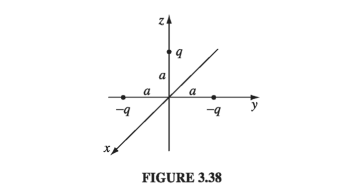
We’ll get to the electric field by writing down the multipole expansion of the potential, and then using the approximate potential to get the electric field. The total charge is -q, so the monopole term will be
\[V_{mon} = \frac{1}{4 \pi \epsilon_0} \frac{1}{r} (-q)\]The dipole moment is given by
\[\begin{aligned} \vec{p} & = \sum_{i=1} ^3 q_i \vec{r_i} \\ & = (-q) a \vu{y} + (-q) a (-\vu{y}) + q a \vu{z} \\ & = qa \vu{z} \end{aligned}\]The dipole term in the multipole expansion of V is then
\[\begin{aligned} V_{dip} & = \frac{1}{4 \pi \epsilon_0} \frac{\vec{p} \cdot \vu{r}}{r^2} \\ & = \frac{1}{4 \pi \epsilon_0} \frac{q a \vu{z} \cdot \vu{r}}{r^2} \\ & = \frac{1}{4 \pi \epsilon_0} \frac{q a \cos \theta}{r^2} \end{aligned}\] \[V(r, \theta) \approx \frac{q}{4 \pi \epsilon_0 } \left( - \frac{1}{r} + \frac{a \cos \theta}{r^2} \right)\]The field is given by
\[\vec{E} = - \grad V \approx \frac{q}{4 \pi \epsilon_0} \left( - \frac{1}{r^2} \vu{r} + \frac{2 a \cos \theta \vu{r}}{r^3} \vu{r} + \frac{a}{r^3} \sin \theta \vu{\theta} \right)\]