\[\]

Pretty much entirely based on this paper: Electromagnetic extension of the Dory– Guest–Harris instability as a benchmark for Vlasov–Maxwell continuum kinetic simulations of magnetized plasmas

Closed Integral Form of Dispersion Relation #

Iman’s done a great job deriving a closed-form integral representation of the dispersion relation for the Dory-Guest-Harris instability. The trick to computing solutions to the dispersion relation is in getting all of the the normalization correct and computing the correct quadrature across both integrals (over $v_\perp$ and $\theta$).

The DGH dispersion relation is derived by perturbing Vlasov-Maxwell system about a spatially uniform equilibrium state $ f_s ^0 (v) $ in a uniform magnetic field $ B^0 $, leading to equilibrium cyclotron motion. We linearize the Vlasov-Maxwell system and analyze the equilibrium response.

Let $ B_0 $ be in the $ \hat{z} $ direction. We work in a cylindrical coordinate system such that

$$ \vec v = v_\perp \cos \phi \hat{x} + v_\perp \sin \phi \hat{y} + v_\parallel \hat{z} $$

Without loss of generality, we rotate the coordinate frame such that

$$ \vec k = k_\perp \hat{x} + k_\parallel \hat{z} $$

The $ v_\parallel $ component de-couples, and we are not interested, so let $v_\parallel = 0$. Would need to be re-introduced for e.g. 2D3V or 3D3V situation, but we will only consider 1D2V here.

After some hard-fought applied mathematics, we get the electromagnetic dispersion relation as

$$ D(\omega, k_\perp) = K_{11} \left( K_{22} - \frac{(\omega_p \tau)^2 k_\perp ^2}{(\omega_c \tau)^2 \omega ^2} \right) - K_{12} K_{21} $$

where

$$ K_{11} = 1 + \chi_{11} $$

$$ K_{12} = \chi_{12} $$

$$ K_{21} = \chi_{21} $$

$$ K_{22} = 1 + \chi_{22} $$

\[\chi = - \frac{2 \pi (\omega_p \tau)^2}{\omega (\omega_c \tau)} \sum_s \frac{\omega_{p, s} ^2}{\omega_{c, s}} \sum_{n = - \infty}^{\infty} \int_0 ^{\infty} \frac{\partial F_s ^0}{\partial v_\perp} \begin{bmatrix} \frac{n^2}{\beta_s ^2} J_n ^2 (\beta_s) & i \frac{n}{\beta_s} J_n (\beta_s) J_n ^\prime (\beta_s) \\\\ - i \frac{n}{\beta_s} J_n(\beta_s) J_n ^\prime(\beta_s) & J_n ^\prime (\beta_s) J_n ^\prime (\beta_s) \end{bmatrix} \frac{v_\perp ^2}{n - \alpha _s} \, d v_\perp\]

$$ \alpha _s \equiv \frac{\omega}{(\omega _c \tau) \omega _{c, s}} $$

$$ \beta_s \equiv \frac{k_\perp v_\perp}{(\omega_c \tau) \omega_{c, s}} $$

$$ F_s ^0 \equiv \frac{f_s ^0}{n_s} $$

$$ \omega_{p, s}^2 \equiv \frac{Z_s ^2 n_s }{A_s} $$

$$ \omega_{c, s} \equiv \frac{Z_s}{A_s} B^0 $$

Manipulation using Lerche-Newberger sum rule, we can get

\[\chi = -\frac{2 \pi (\omega_p \tau)^2}{\omega (\omega_c \tau)} \sum_s \frac{\omega_{p, s}^2}{\omega_{c, s}} \int_0 ^\infty \frac{\partial F_s ^0 }{\partial v_\perp} \begin{bmatrix} \frac{\alpha_s}{\beta_s ^2} (1 - Q_s) & - \frac{i}{2 \beta_s} Q_s ^\prime \\ \frac{i}{2 \beta_s} Q_s ^\prime & - \left( \frac{\pi}{\sin (\pi \alpha_s)} J_{- \alpha_s} ^\prime (\beta_s) J_{\alpha_s} ^\prime (\beta_s) + \frac{\alpha_s}{\beta_s ^2} \right) \end{bmatrix} v_\perp ^2 \, d v_\perp\]

where

$$ Q_s \equiv \frac{\pi \alpha_s}{\sin (\pi \alpha_s)} J_{- \alpha_s }(\beta_s) J_{\alpha_s}(\beta_s) $$

$$ Q_s ^\prime \equiv \frac{\pi \alpha_s}{\sin (\pi \alpha_s)} \frac{\partial}{\partial \beta_s} \left[ J_{- \alpha_s}(\beta_s) J_{\alpha_s}(\beta_s) \right] $$

We can re-cast the Bessel function products in terms of integrals of real low-order Bessel functions:

$$ J_{- \alpha_s}(\beta) J_{\alpha_s}(\beta) = \frac{2}{\pi} \int_0 ^{\pi / 2} J_0 (2 \beta \cos \theta) \cos (2 \alpha_s \theta) d \theta $$

$$ \frac{\partial}{\partial \beta} [J_{-\alpha_s} (\beta) J_{\alpha_s} (\beta)] = - \frac{4}{\pi} \int_0 ^{\pi / 2} J_1 (2 \beta \cos \theta) \cos \theta \cos (2 \alpha_s \theta) d \theta $$

$$ J^\prime _{- \alpha_s} (\beta) J^\prime _{\alpha_s} (\beta_s) = \frac{1}{\pi} \left[ \int_0 ^{\pi / 2} \cos (2 \alpha_s \theta) [J_2 (2 \beta \cos \theta) - J_0(2 \beta \cos \theta) \cos (2 \theta)] d \theta - \frac{\alpha_s}{\beta^2} \sin (\pi \alpha_s)\right] $$

We are looking at a single-species picture, and we choose electrons. That means that

$$ A_s = 1 $$ $$ Z_s = -1 $$ $$ n = 1 $$

We choose (the cases in https://doi.org/10.1016/j.jcp.2014.08.014):

$$ B^0 = 1 $$ $$ v_\perp ^0 = \sqrt{2} $$ $$ f^0 (v_\perp) \equiv \frac{1}{\pi \alpha_\perp ^2 j!} \left(\frac{v_\perp ^2}{\alpha_\perp ^2} \right)^j e^{- v_\perp ^2 / \alpha_\perp ^2} $$

Things I need for integration: #

$$ (\omega_p \tau) = 1 $$ $$ (\omega_c \tau) = (\omega_p / \omega_c)^{-1} $$ $$ \omega = \text{(free parameter)} $$ $$ \omega_{p_s} \equiv \frac{Z_s ^2 n_s}{A_s} = 1 $$ $$ \omega_{c_s} \equiv \frac{Z_s}{A_s} B^0 = -1 $$

\[\partial F^0 _s / \partial v_\perp = \frac{1}{\pi \alpha_\perp ^2 j!} \frac{2 v_\perp}{\alpha_\perp ^2} e^{- v_\perp ^2 / \alpha_\perp ^2} \left( \frac{v_\perp ^2}{\alpha_\perp ^2}\right)^{j-1} \left[j - \frac{v_\perp ^2}{\alpha_\perp ^2} \right]\]

$$ n = 1 $$

$$ \omega_p / \omega_c = \left(\frac{n_0 m_0}{\epsilon_0 B_0 ^2} \right)^{1/2} = \text{(free parameter)} $$

($\omega_p / \omega_c$ dictates the relative strength of $B$ to $E$)

We express $k_\perp$ in terms of a normalized wavenumber $\tilde{k}$:

$$ \tilde{k} \equiv k_\perp v_{\perp, 0} \frac{\omega_p}{\omega_c} \quad \text{(free parameter)} $$

$$ \rightarrow \beta_s = - \frac{\tilde{k} v_{\perp}}{v_{\perp, 0}} $$

Now let’s try to factor out some of the mess from $\chi$. Substituting in our single-species values for $(\omega_{p, s})$, $(\omega_{c, s})$, $(\omega_p \tau)$, and $(\omega_c \tau)$:

\[\begin{aligned} \chi & = & -\frac{2 \pi (\omega_p \tau)^2}{\omega (\omega_c \tau)} \frac{\omega_{p, s}^2}{\omega_{c, s}} \int_0 ^\infty \frac{\partial F_s ^0 }{\partial v_\perp} v_\perp ^2 \begin{bmatrix} \frac{\alpha_s}{\beta_s ^2} (1 - Q_s) & - \frac{i}{2 \beta_s} Q_s ^\prime \\ \frac{i}{2 \beta_s} Q_s ^\prime & - \left( \frac{\pi}{\sin (\pi \alpha_s)} J_{- \alpha_s} ^\prime (\beta_s) J_{\alpha_s} ^\prime (\beta_s) + \frac{\alpha_s}{\beta_s ^2} \right) \end{bmatrix} \, d v_\perp \\ & = & -\frac{2 \pi (\omega_p \tau)^2}{\omega (\omega_c \tau)} \frac{\omega_{p, s}^2}{\omega_{c, s}} \int_0 ^\infty \frac{\partial F_s ^0 }{\partial v_\perp} \frac{v_\perp ^2}{\beta_s ^2} \beta_s ^2 \begin{bmatrix} \frac{\alpha_s}{\beta_s ^2} (1 - Q_s) & - \frac{i}{2 \beta_s} Q_s ^\prime \\ \frac{i}{2 \beta_s} Q_s ^\prime & - \left( \frac{\pi}{\sin (\pi \alpha_s)} J_{- \alpha_s} ^\prime (\beta_s) J_{\alpha_s} ^\prime (\beta_s) + \frac{\alpha_s}{\beta_s ^2} \right) \end{bmatrix} \, d v_\perp \\ & = & -\frac{2 \pi (\omega_p \tau)^2}{\omega (\omega_c \tau)} \frac{\omega_{p, s}^2}{\omega_{c, s}} \frac{(\omega_c \tau)^2 \omega_{c, s}^2}{k_\perp ^2} \int_0 ^\infty \frac{\partial F_s ^0 }{\partial v_\perp} \beta_s ^2 \begin{bmatrix} \frac{\alpha_s}{\beta_s ^2} (1 - Q_s) & - \frac{i}{2 \beta_s} Q_s ^\prime \\ \frac{i}{2 \beta_s} Q_s ^\prime & - \left( \frac{\pi}{\sin (\pi \alpha_s)} J_{- \alpha_s} ^\prime (\beta_s) J_{\alpha_s} ^\prime (\beta_s) + \frac{\alpha_s}{\beta_s ^2} \right) \end{bmatrix} \, d v_\perp \\ & = & -\frac{2 \pi v_{\perp, 0}^2 (\omega_p / \omega_c)}{\tilde{k}^2 \omega} \int_0 ^\infty \frac{\partial F_s ^0 }{\partial v_\perp} \beta_s ^2 \begin{bmatrix} \frac{\alpha_s}{\beta_s ^2} (1 - Q_s) & - \frac{i}{2 \beta_s} Q_s ^\prime \\ \frac{i}{2 \beta_s} Q_s ^\prime & - \left( \frac{\pi}{\sin (\pi \alpha_s)} J_{- \alpha_s} ^\prime (\beta_s) J_{\alpha_s} ^\prime (\beta_s) + \frac{\alpha_s}{\beta_s ^2} \right) \end{bmatrix} \, d v_\perp \\ & = & -\frac{2 \pi v_{\perp, 0}^2 (\omega_p / \omega_c)}{\tilde{k}^2 \omega} \int_0 ^\infty \frac{\partial F_s ^0 }{\partial v_\perp} \begin{bmatrix} \alpha_s (1 - Q_s) & - \frac{i \beta_s}{2} Q_s ^\prime \\ \frac{i \beta_s}{2} Q_s ^\prime & - \left( \frac{\pi \beta_s ^2}{\sin (\pi \alpha_s)} J_{- \alpha_s} ^\prime (\beta_s) J_{\alpha_s} ^\prime (\beta_s) + \alpha_s \right) \end{bmatrix} \, d v_\perp \\ \end{aligned}\]

Let’s re-write things a bit for simplicity:

\[R_{ij} = \begin{bmatrix} \alpha _s (1 - Q _s) & - \frac{i \beta _s}{2} Q ^\prime _s \\\\ \frac{i \beta _s}{2} Q^\prime _s & - \beta _s ^2 \left( \frac{\pi}{\sin (\pi \alpha _s)} J_{- \alpha _s} ^\prime (\beta _s) J_{\alpha _s} ^\prime (\beta _s) + \frac{\alpha _s}{\beta _s ^2} \right) \end{bmatrix}\]

Using Bessel function identities,

$$ R_{22} = - \beta_s ^2 \left( \frac{\pi}{\sin (\pi \alpha_s)} J_{- \alpha_s} ^\prime (\beta_s) J_{\alpha_s} ^\prime (\beta_s) + \frac{\alpha_s}{\beta_s ^2} \right) \\ = - \beta_s ^2 \left(\frac{\pi}{\sin (\pi \alpha_s)} \left[ \frac{1}{\pi} \left( \int _0 ^{\pi / 2} \cos (2 \alpha_s \theta) \left[ J_2(2 \beta_s \cos \theta) - J_0 (2 \beta_s \cos \theta) \cos (2 \theta) \right] d \theta - \frac{\alpha_s}{\beta_s ^2} \sin (\pi \alpha_s) \right) \right] + \frac{\alpha_s}{\beta_s} \right) \\ = - \frac{\beta_s ^2}{\sin (\pi \alpha_s)} \int_0 ^{\pi / 2} \cos (2 \alpha_s \theta) \left[ J_2(2 \beta_s \cos \theta) - J_0 (2 \beta_s \cos \theta) \cos (2 \theta) \right] \, d \theta $$

Still not pretty, but we can give it a try. Let’s try using https://github.com/JuliaMath/QuadGK.jl to compute the improper integral over $v_\perp$, and use Gauss-Legendre quadrature to compute the interior $\theta$ integrals.

using Pkg
Pkg.add("Plots")
Pkg.add("PythonPlot")
Pkg.add("HDF5")
Pkg.add("Optim")
Pkg.add("LaTeXStrings")
Pkg.add(url="https://github.com/JuliaApproximation/FastGaussQuadrature.jl")
Pkg.add(url="https://github.com/JuliaMath/Bessels.jl.git")
Pkg.add(url="https://github.com/JuliaMath/QuadGK.jl")
using Bessels  # besselj
using FastGaussQuadrature  # compute gauss-legendre points
using HDF5  # store/read from file
using LaTeXStrings  # Plot formatting
using LinearAlgebra  # dot.()
using Optim  # Newton-Raphson descent to find zeros
using Plots  # Matplotlib metapackage
using QuadGK  # Alternative integrator

# Set plotting backend to matplotlib
pythonplot()
# Set plotting backend to GR
# gr()

# Base.@kwdef is a macro that allows for keyword arguments and default values
Base.@kwdef struct DispersionCase
  id::String
  knorm::Float64
  j::Int
  width::Float64
  wpwc::Float64
  guesses::Vector{Vector{Float64}}
end

const case_a = DispersionCase(id="A", knorm=3.15, j=6, width=sqrt(1/3), wpwc=20.0, guesses=[[0.0,0.5]])
const case_b = DispersionCase(id="B", knorm=4.64, j=6, width=sqrt(1/3), wpwc=20.0, guesses=[[1.0, 0.3]])
const case_c = DispersionCase(id="C", knorm=2.12, j=2, width=1.0, wpwc=10.0, guesses=[[0.8, 0.12]])
const case_d = DispersionCase(id="D", knorm=2.12, j=1, width=sqrt(2), wpwc=1.0, guesses=[[1.5, 0.0]])
const cases = [case_a, case_b, case_c, case_d]

function solve_em_dispersion(;knorm, j, width, wpwc, wr, wi)
  v_0 = sqrt(j) * width

  function dF0_dv(v)
    return 2 * v / (pi * width^4 * factorial(j)) * exp(-v^2 / width^2) * (v^2 / width^2)^(j - 1) * (j - (v^2 / width^2))
  end

  quad_samples, quad_weights = gausslegendre(100);
  
  # Transform from [-1, 1] to [0, 20]
  v_samples = @. 10.0 * (1.0 + quad_samples)
  v_weights = @. 10.0 * quad_weights
  
  # Transform from [-1, 1] to [0, pi/2] for interior quadrature calculations
  theta = 0.25 * pi * (1.0 .+ quad_samples)
  theta_weights = 0.25 * pi .* quad_weights
  
  function Q_s(alpha, beta)
    return (2 * alpha / sin(pi * alpha)) * dot(theta_weights, besselj0.(2 * beta * cos.(theta)) .* cos.(2 * alpha .* theta))
  end
  
  function Qp_s(alpha, beta)
    return -(4 * alpha / sin(pi * alpha)) * dot(theta_weights, besselj1.(2 * beta * cos.(theta)) .* cos.(theta) .* cos.(2 * alpha .* theta))
  end
  
  function R22(alpha, beta)
    return (-beta^2 / sin(pi * alpha)) * dot(theta_weights, cos.(2 * alpha * theta) .* (besselj.(2, 2 * beta * cos.(theta)) - besselj0.(2 * beta * cos.(theta)) .* cos.(2 * theta)))
  end
  
  # quadgk integration tolerance
  rtol = 1e-10
  
  function r11(w)
    alpha = -w * wpwc
    function integrand(v)
      beta = -knorm * v / v_0
      return dF0_dv(v) * alpha * (1 - Q_s(alpha, beta))
    end
    I, err = quadgk(integrand, 0.0, Inf, rtol=rtol)
    return I
  end
  
  function r12(w)
    alpha = -w * wpwc
    function integrand(v)
      beta = -knorm * v / v_0
      return -dF0_dv(v) * 0.5 * im * beta * Qp_s(alpha, beta)
    end
    I, err = quadgk(integrand, 0.0, Inf, rtol=rtol)
    return I
  end
  
  function r22(w)
    alpha = -w * wpwc
    function integrand(v)
      beta = -knorm * v / v_0
      return -dF0_dv(v) * (-beta^2 / sin(pi * alpha)) * dot(theta_weights, cos.(2 * alpha * theta) .* (besselj.(2, 2 * beta * cos.(theta)) - besselj0.(2 * beta * cos.(theta)) .* cos.(2 * theta)))
    end
    I, err = quadgk(integrand, 0.0, Inf, rtol=rtol)
    return I
  end
  
  function dispersion(w)
    coeff = 2.0 * pi * v_0^2 * wpwc / (knorm^2 * w)
    x11 = coeff * r11(w)
    x12 = coeff * r12(w)
    x22 = coeff * r22(w)
    k11 = 1.0 + x11
    k12 = x12
    k21 = -x12
    k22 = 1.0 + x22
    D = k11 * (k22 + knorm^2 / (v_0 ^2 * w^2)) - k12 * k21
    return D
  end

  w = wr + im * wi
  return dispersion(w)

end

function solve_es_dispersion(;knorm, j, width, wpwc, wr, wi)
  
end

function plot_contours_from_file(filename)
  fid = HDF5.h5open(filename, "r")
  x = HDF5.read(fid["w_r"])
  y = HDF5.read(fid["w_i"])
  D = HDF5.read(fid["D"])
  case_id = HDF5.read(fid["caseId"])
  wpwc = HDF5.read(fid["wpwc"])
  close(fid)

  z = abs.(D)
  min_log = minimum(z) / maximum(z)
  min_level = trunc(Int, log(min_log))
  levels = -min_level:0
  colorbar_labels = [L"10^{%$i}" for i in levels]
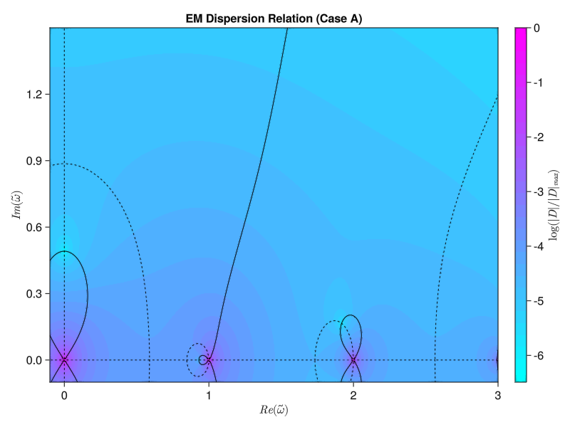
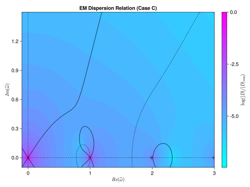
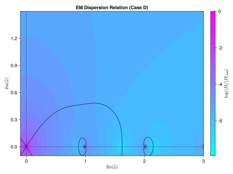
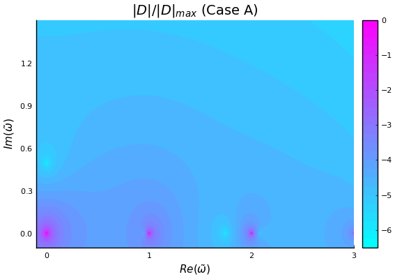
  plt = contourf(x, y, log10.(z ./ maximum(z)), levels=30, color=:cool, colorbar_ticks=(levels, colorbar_labels))
  title!(L"$|D|/|D|_{max}$ (Case " * case_id * ")")
  xlabel!(L"Re(\tilde{\omega})")
  ylabel!(L"Im(\tilde{\omega})")
  savefig(plt, "julia-dgh-case" * case_id * ".pdf")
  display(plt)
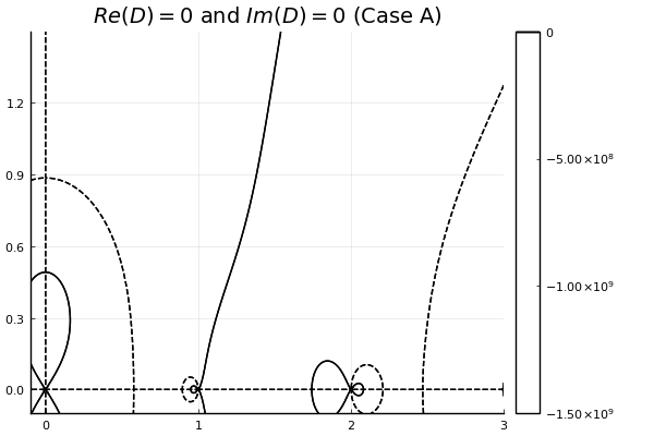
  contour_plt = contour(x, y, real.(D), levels=[0.0, 0.001], c=[:black], ls=[:solid])
  contour!(contour_plt, x, y, imag.(D), levels=[0.0, 0.001], c=[:black], ls=[:dash])
  title!(L"$Re(D)=0$ and $Im(D)=0$ (Case " * case_id * ")")
  display(contour_plt)
end

function run_case(case, file_base_name, num_pts)
  filename = file_base_name * "-" * case.id * ".h5"
  fid = HDF5.h5open(filename, "w")
  fid["caseId"] = case.id
  fid["knorm"] = case.knorm
  fid["j"] = case.j
  fid["width"] = case.width
  fid["wpwc"] = case.wpwc
  x = range(-0.1, 3.0, length=num_pts)
  y = range(-0.1, 1.5, length=num_pts)
  fid["w_r"] = collect(x)
  fid["w_i"] = collect(y)
  function em_dispersion(wr, wi)
    return solve_em_dispersion(knorm=case.knorm, j=case.j, width=case.width, wpwc=case.wpwc, wr=wr, wi=wi)
  end
  println("Running case ", case.id, " over ", num_pts^2, " total points..." )
  D = @. em_dispersion(x' ./ case.wpwc, y ./ case.wpwc)
  fid["D"] = D
  close(fid)
  println("Finished. Writing to file ", filename)
  return filename
end

filename = run_case(cases[1], "data", 320)
plot_contours_from_file(filename)

It’s very close! The basic anatomy looks to be nearly correct. Most importantly, the fastest-growing mode (the zero with the largest imaginary frequency component) that we see appears to be near the expected $\tilde{\omega} = 0.0 + 0:4912i$:

img/research/dgh/dispersion-fail-julia-1.png

We can confirm by running a minimization scheme near the zero to get a precise value. I’ll use the Optim.jl library to perform the descent minimization:


function find_zero(case)
  function em_dispersion(w)
    return abs(solve_em_dispersion(knorm=case.knorm, j=case.j, width=case.width, wpwc=case.wpwc, wr=w[1], wi=w[2]))
  end
  println("========== Case ", case.id, " ==========")
  for guess in case.guesses
    start = [guess[1] / case.wpwc, guess[2] / case.wpwc]
    println("Searching for zero near w = ", guess[1], " + ", guess[2], "i")
    result = optimize(em_dispersion, start, Optim.Options(x_tol = 1e-6))
    println("Case ", case.id, ":")
    display(result)
    println("Did we find a root? Maybe! We think there is a root at:")
    println("w = ", round(Optim.minimizer(result)[1] * case.wpwc, digits=5), " + ", round(Optim.minimizer(result)[2] * case.wpwc, digits=5), "i")
  end
end
find_zero(cases[1])

========== Case A ==========
Searching for zero near w = 0.0 + 0.5i
 * Status: success

 * Candidate solution
    Final objective value:     2.739900e-08

 * Found with
    Algorithm:     Nelder-Mead

 * Convergence measures
    √(Σ(yᵢ-ȳ)²)/n ≤ 1.0e-08

 * Work counters
    Seconds run:   3  (vs limit Inf)
    Iterations:    94
    f(x) calls:    184
Case A:
Did we find a root? Maybe! We think there is a root at:
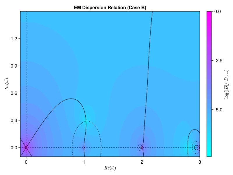
w = 0.0 + 0.49123i

So far so good! But I am very suspicious that I don’t see any other growing modes. From Iman’s paper I would expect to see another solution near $\tilde{\omega} = 1.9 + 0.2i$ Let’s try a different case, setting $\tilde{k} = 4.65$. This is “Case B” in the paper, and I expect a solution at $\tilde{\omega} = 1.0363 + 0.2900i$:

========== Case B ==========
Searching for zero near w = 1.0 + 0.3i
 * Status: success

 * Candidate solution
    Final objective value:     2.216717e-08

 * Found with
    Algorithm:     Nelder-Mead

 * Convergence measures
    √(Σ(yᵢ-ȳ)²)/n ≤ 1.0e-08

 * Work counters
    Seconds run:   3  (vs limit Inf)
    Iterations:    89
    f(x) calls:    175
Case B:
Did we find a root? Maybe! We think there is a root at:
w = 1.03461 + 0.28968i

Hmm, that is much further off than I would like. Decreasing the tolerance for the QuadGK integrals does not change the result, and increasing the number of Gauss-Legendre quadrature points also makes no difference.

How about we try doing the v integrals by quadrature as well?

No quadrature, two contour plots with 400pts each: 16.7 sec Quadrature, two contour plots with 400pts each: 6.1 sec!

Back to the original attempt code, evaluating with 1600pts each and threading I get 30.7s with QuadGK, and 6.3s with my own quadrature! Let’s definitely use that instead:

function solve_em_dispersion(; knorm, j, width, wpwc, w_array)
  # All normalization parameters
  Ze = -1.0  # Charge ratio for species
  Ae = 1.0  # Mass ratio for species
  wptau = 1.0  # Time normalization
  wctau = 1.0 / wpwc  # omega_c * tau
  Omega = Ze / Ae / wpwc  # Species-dependent cyclotron frequency
  B0z = 1.0  # Magnetic field magnitude
  vp0 = sqrt(2.0)  # Ring distribution peak velocity
  k = knorm / vp0 / wpwc  # Normalized k
  ne = 1.0  # Species density
  wce = Ze / Ae * B0z  # Normalized cyclotron frequency
  wp2 = Ze^2 * ne / Ae  # Normalized plasma frequency squared

  beta = @. k * v_perp / wce / wctau
  f0prime = @. 2 * v_perp / (pi * width^4 * factorial(j)) * exp(-v_perp^2 / width^2) * (v_perp^2 / width^2)^(j - 1) * (j - (v_perp^2 / width^2))

  Q = similar(beta, ComplexF64)  # Initialize empty Q
  Qprime = similar(beta, ComplexF64)  # Initialize empty Q'
  jprime_ma_jprime_pa = similar(beta, ComplexF64)  # Initialize empty J'_-a(b)*J'_+a(b)
  D = similar(w_array, ComplexF64)  # Output array for each input w

  for (idx, w) in enumerate(w_array)
    alpha = w / wce / wctau  
    sine_factor = pi * alpha / sin(pi * alpha)
    cos_2_a_theta = @. cos(2 * alpha * theta)

    for ii in 1:length(beta)
      two_beta_cos_theta = (2.0 * beta[ii]) .* cos_theta
      Q[ii] = sine_factor * 2.0 / pi * sum(theta_weights .* (besselj0.(two_beta_cos_theta) .* cos_2_a_theta))
      Qprime[ii] = sine_factor * -4.0 / pi * sum(theta_weights .* (besselj1.(two_beta_cos_theta) .* cos_theta .* cos_2_a_theta))
      jprime_ma_jprime_pa[ii] = 1.0 / pi * (sum(theta_weights .* (cos_2_a_theta .* (besselj.(2, two_beta_cos_theta) .- besselj0.(two_beta_cos_theta) .* cos_2_theta))) - alpha .* sin.(pi .* alpha)/ beta[ii]^2)
    end

    v_integrand_11 = @. - f0prime * (alpha / beta^2 * (1.0 - Q)) * v_perp^2
    v_integrand_12 = @. f0prime * (im / 2.0 / beta * Qprime) * v_perp^2
    v_integrand_22 = @. f0prime * (sine_factor / alpha * jprime_ma_jprime_pa + alpha / beta^2) * v_perp^2
    coeff = wptau^2 / wctau * 2.0 * pi * wp2 / w / wce
    chi_xx = coeff * sum(v_weights .* v_integrand_11)
    chi_xy = coeff * sum(v_weights .* v_integrand_12)
    chi_yy = coeff * sum(v_weights .* v_integrand_22)
    K_xx = 1.0 + chi_xx
    K_xy = chi_xy
    K_yx = - K_xy
    K_yy = 1.0 + chi_yy

    D[idx] = K_xx * (K_yy - wptau^2 / w^2 / wctau^2 * k^2) - K_xy * K_yx
  end
  return D
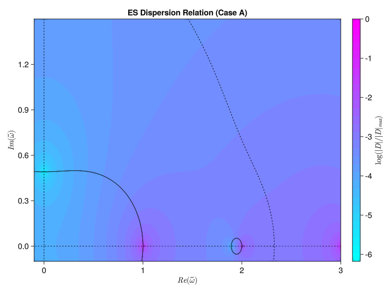
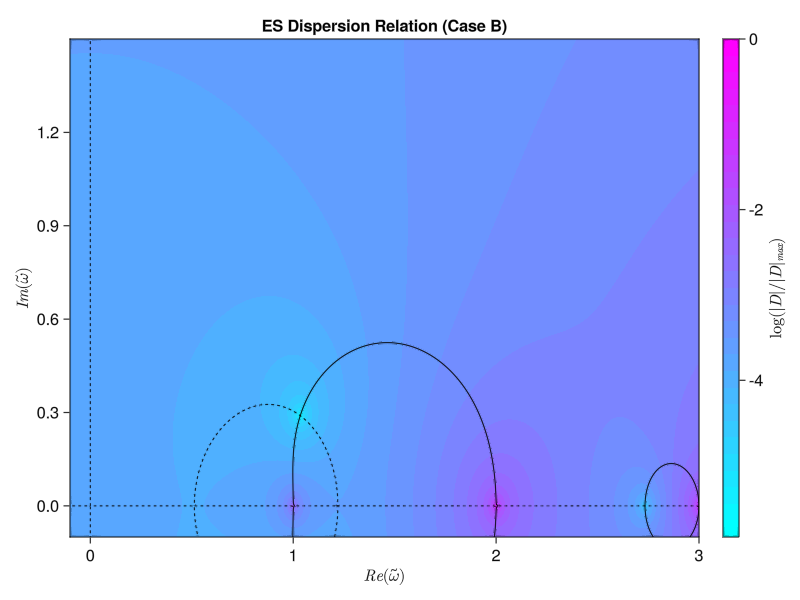
end

We’ve got to use some for loops instead of straight broadcasting to do the double integral properly, but now we get the same results as the paper! Similarly, we should be able to compute the electrostatic version using either the simplified single-species version from Tartaronis or the full multi-species version from Vogman. We’ll use the latter:

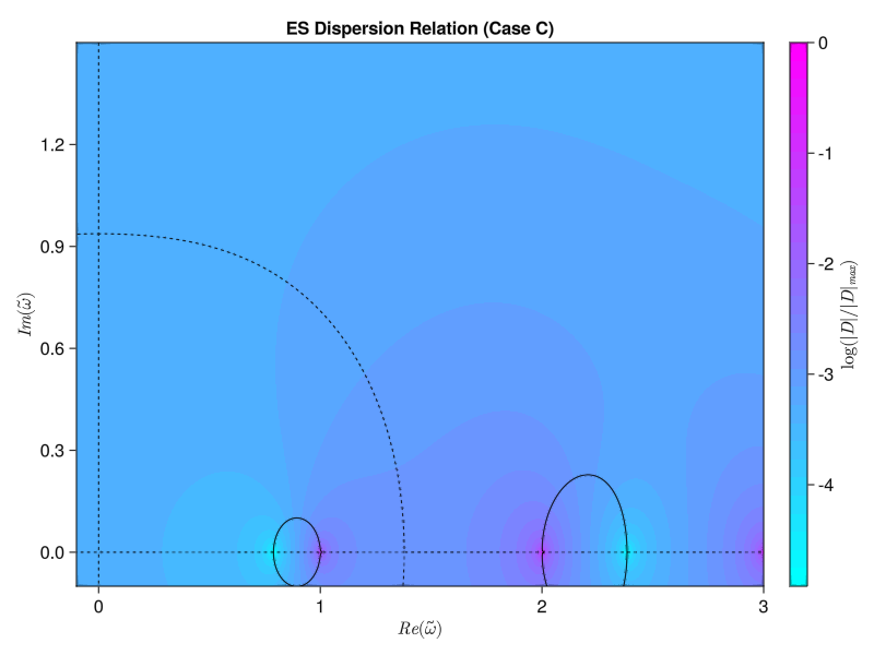
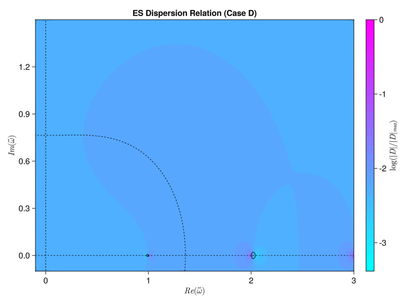
\[D(\omega, k_\perp) = 1 + \sum_s M_s \frac{\omega_p ^2}{\omega_c ^2} \int_0 ^\pi \frac{\sin(\omega \tau / \Omega_{cs})}{\sin(\omega \pi / \Omega_{cs})} \sin (\tau) F_0 (\tau + \pi) \dd \tau = 0\] where \[F_0 (\tau) = \int_0 ^\infty f_{s, 0} (v_\perp) J_0 \left( 2 \frac{k_\perp v_\perp}{\Omega_{cs}} \sin(\frac{\tau}{2})\right) 2 \pi v_\perp \dd v_\perp\] \[\Omega_{cs} \equiv \frac{Z_s \omega_c}{M_s \omega_p}\]

function solve_es_dispersion(; knorm, j, width, wpwc, w_array)
  # All normalization parameters
  Ze = -1.0  # Charge ratio for species
  Ae = 1.0  # Mass ratio for species
  wptau = 1.0  # Time normalization
  wctau = 1.0 / wpwc  # omega_c * tau
  Omega = Ze / Ae / wpwc  # Species-dependent cyclotron frequency
  B0z = 1.0  # Magnetic field magnitude
  vp0 = sqrt(2.0)  # Ring distribution peak velocity
  k = knorm / vp0 / wpwc  # Normalized k
  ne = 1.0  # Species density
  wce = Ze / Ae * B0z  # Normalized cyclotron frequency
  wp2 = Ze^2 * ne / Ae  # Normalized plasma frequency squared
  
  # Initial distribution
  vp_alpha = v_perp ./ width
  f0 = @. ne / (pi * width^2 * factorial(j)) * (vp_alpha)^(2*j) * exp(- vp_alpha ^2)

  z = @. k * v_perp / Omega / B0z
  D = similar(w_array, ComplexF64)
  for (idx, w) in enumerate(w_array)
    w_alpha = w / Omega / B0z
    tau_int = similar(z, ComplexF64)
    for ii in 1:length(z)
      # tau = range(0.0, pi, 100)
      tau_integrand = @. sin(w_alpha * tau) / sin(w_alpha * pi) * sin(tau) * besselj0(2 * z[ii] * sin((tau + pi)/2))
      # tau_int[ii] = trapz(tau, tau_integrand)
      tau_int[ii] = sum(tau_weights .* tau_integrand)
    end
    v_integrand = @. f0 * tau_int * v_perp
    D[idx] = 1.0 + 2.0 * pi * Ze^2 / Ae / Omega^2 * sum(v_weights .* v_integrand)
  end
  return D
end

Electromagnetic	Electrostatic