

3.2: The Method of Images

3.1.1: The Classic Image Problem

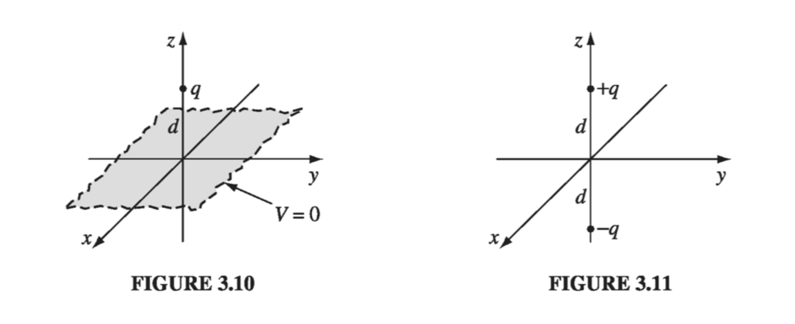
Suppose a point charge q is held a distance d above an infinite grounded conducting plane (Fig. 3.10). Question: what is the potential in the region above the plane? It's not just $(1/4 \pi \epsilon_0) q / \gr$, for q will induce a certain amount of negative charge on the nearby surface of the conductor; the total potential is due in part to q directly, and in part to this induced charge. But how can we possibly calculate the potential, when we don't know how much charge is induced or how it is distributed?

From a mathematical point of view, our problem is to solve Poisson's equation in the region $z > 0$, with a single point charge q at $(0, 0, d)$, subject to the boundary conditions

1. $V = 0$ when $z = 0$ (since the conducting plane is grounded)
2. $V \rightarrow 0$ far from the charge (that is, for $x^2 + y^2 + z^2 \gg d^2$

The first uniqueness theorem (actually, its corollary) guarantees that there is only one function that meets these requirements. If by trick or clever guess we can discover such a function, it's got to be the answer. Trick: Forget about the actual problem; we're going to study a completely different situation. This new configuration consists of two point charges, $+q$ at $(0, 0, d)$ and $-q$ at $(0, 0, -d)$, and no conducting plane (Fig. 3.11). For this configuration I can easily write down the potential: $$V(x, y, z) = \frac{1}{4 \pi \epsilon_0} \left[ \frac{q}{\sqrt{x^2 + y^2 + (z - d)^2 }} - \frac{q}{\sqrt{x^2 + y^2 + (z + d)^2}} \right] \label{3.9} \tag{3.9}$$ It follows that

1. $V = 0$ when $z = 0$
2. $V \rightarrow 0$ for $x^2 + y^2 + z^2 \gg d^2$

and the only charge in the region $z > 0$ is the point charge $+q$ at $(0, 0, d)$. But these are precisely the conditions of the original problem! Evidently the second configuration happens to produce exactly the same potential as the first configuration, in the "upper" region $z \geq 0$. (The "lower" region, $z < 0$, is completely different, but who cares? The upper part is all we need.) Conclusion: The potential of a point charge above an infinite grounded conductor is given by $\eqref{3.9}$, for $z > 0$.

Notice the crucial role played by the uniqueness theorem in this argument: without it, no one would believe this solution, since it was obtained for a completely different charge distribution. But the uniqueness theorem certifies it: If it satisfies Poisson's equation in the region of interest, and assumes the correct value at the boundaries, then it must be right.

3.2.2: Induced Surface Charge

Now that we know the potential, it is a straightforward matter to compute the surface charge $\sigma$ induced on the conductor. According to Eq. 2.49, $$\sigma = - \epsilon_0 \pdv{V}{n}$$ where $\partial V / \partial n$ is the normal derivative of V at the surface. In this case the normal direction is the z direction, so $$\sigma = \left. - \epsilon_0 \pdv{V}{z} \right|_{z = 0}$$ From Eq. 3.9 $$\pdv{V}{z} = \frac{1}{4 \pi \epsilon_0} \left[ \frac{-q (z - d)}{[x^2 + y^2 + (z - d)^2]^{3/2}} + \frac{q(z + d)}{[x^2 + y^2 + (z + d)^2 ]^{3/2}} \right]$$ so $$\sigma(x, y) = \frac{-qd}{2 \pi (x^2 + y^2 + d^2)^{3/2}} \label{3.10} \tag{3.10}$$ As expected, the induced charge is negative (assuming q is positive) and greatest at $x = y = 0$.

While we're at it, let's compute the total induced charge $$Q = \int \sigma \dd{a}$$ This integral, over the xy plane, could be done in Cartesian coordinates, with $\dd{a} = \dd{x} \dd{y}$, but it's easier to use polar coordinates $(r, \phi)$, with $r^2 = x^2 + y^2$ and $\dd{a} = r \dd{r} \dd{\phi}$. Then $$\sigma(r) = \frac{-qd}{2 \pi (r^2 + d^2)^{3/2}}$$ and $$Q = \int_{0} ^{2\pi} \int_{0} ^{\infty} \frac{-qd}{2 \pi (r^2 + d^2)^{3/2}} r \dd{r} \dd{\phi} = \left. \frac{qd}{\sqrt{r^2 + d^2}} \right|_{0} ^{\infty} = -q \label{3.11} \tag{3.11}$$

The total charge induced on the plane is $-q$, as (with benefit of hindsight) you can perhaps convince yourself it had to be.

3.2.3: Force and Energy

The charge $q$ is attracted toward the plane, because of the negative induced charge. Let's calculate the force of attraction. Since the potential in the vicinity of $q$ is the same as in the analog problem (the one with $+q$ and $-q$ but no conductor), so also is the field and, therefore, the force $$\vec{F} = -\frac{1}{4 \pi \epsilon_0} \frac{q^2}{(2d)^2} \vu{z} \label{3.12} \tag{3.12}$$

Beware: It is easy to get carried away, and assume that everything is the same in the two problems. Energy, however, is not the same. With the two point charges and no conductor, Eq. 2.42 gives $$W = - \frac{1}{4 \pi \epsilon_0} \frac{q^2}{2d}$$ But for a single charge and conducting plane, the energy is half this $$W = - \frac{1}{4 \pi \epsilon_0} \frac{q^2}{4d} \label{3.14} \tag{3.14}$$ Why half? Think of the energy stored in the fields (Eq. 2.45): $$W = \frac{\epsilon_0}{2} \int E^2 \dd{\tau}$$ In the first case, both the upper region $(z > 0)$ and the lower region $(z < 0)$ contribute, and by symmetry they contribute equally. But in the second case, only the upper region contains a nonzero field, and hence the energy is half as great.

Of course, one could also determine the energy by calculating the work required to bring $q$ in from infinity. The force required (to oppose the electrical force in $\eqref{3.12}$ is $(1 / 4 \pi \epsilon_0)(q^2/4z^2) \vu{z}$, so $$\begin{align} W & = & \int _{\infty} ^{d} \vec{F} \cdot \dd{\vec{l}} = \frac{1}{4 \pi \epsilon_0} \int_{\infty} ^d \frac{q^2}{4z^2} \dd{z} \\ & = & \frac{1}{4 \pi \epsilon_0} \left. \left( - \frac{q^2}{4z} \right) \right|_{\infty} ^d = - \frac{1}{4 \pi \epsilon_0} \frac{q^2}{4d} \end{align}$$ As I move $q$ toward the conductor, I do work only on q. It is true that induced charge is moving in over the conductor, but this costs me nothing, since the whole conductor is at potential zero. By contrast, if I simultaneously bring in two point charges (with no conductor), I do work on both of them, and the total is (again) twice as great.

3.2.4: Other Image Problems

The method just described is not limited to a single point charge; any stationary charge distribution near a grounded conducting plane can be treated in the same way, by introducing its mirror image - hence the name method of images. (Remember that the image charges have the opposite sign; this is what guarantees that the xy plane will be at potential zero.) There are also some exotic problems that can be handled in similar fashion; the nicest of these is the following.

Example 3.2

A point charge q is situated a distance a from the center of a grounded conducting sphere of radius R (Fig. 3.12). Find the potential outside the sphere

Solution Examine the completely different configuration, consisting of the point charge q together with another point charge $$q' = - \frac{R}{a} q \label{3.15} \tag{3.15}$$ placed a distance $$b = \frac{R^2}{a} \label{3.16} \tag{3.16}$$ to the right of the center of the sphere (Fig 3.13). No conductor, now - just the two point charges. The potential of this configuration is $$V(\vec{r}) = \frac{1}{4 \pi \epsilon_0} \left( \frac{q}{\gr} + \frac{q'}{\gr '} \right) \label{3.17} \tag{3.17}$$ where $\gr$ and $\gr'$ are the distances from q and q', respectively. Now, it happens (see Prob. 3.8) that this potential vanishes at all points on the sphere, and therefore fits the boundary conditions for our original problem, in the exterior region.

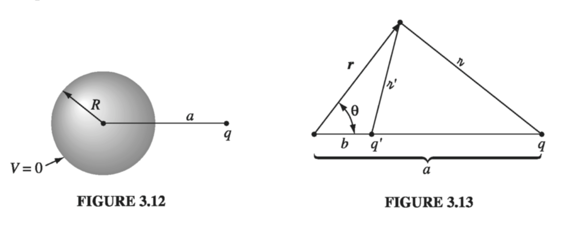
Conclusion: $\eqref{3.17}$ is the potential of a point charge near a grounded conducting sphere. (Notice that b is less than R, so the "image" charge q' is safely inside the sphere - you cannot put image charges in the region where you are calculating V; that would change $\rho$, and you'd be solving Poisson's equation with the wrong source.) In particular, the force of attraction between the charge and the sphere is $$F = \frac{1}{4\pi \epsilon_0} \frac{q q'}{(a - b)^2} = - \frac{1}{4 \pi \epsilon_0} \frac{q^2 R a}{(a^2 - R^2)^2} \label{3.18} \tag{3.18}$$

The method of images is delightfully simple... when it works. But it is as much an art as a science, for you must somehow think up just the right "auxiliary" configuration, and for most shapes this is forbiddingly complicated, if not impossible.